Week 3: Longitudinal Data Analysis using Multilevel Modeling

class: center, middle, inverse, title-slide

# Week 3: Longitudinal Data Analysis using Multilevel Modeling - Nonlinear Change
## Multivariate Statistics and Methodology using R (MSMR) 
### Dan Mirman
### Department of Psychology The University of Edinburgh

---

# Longitudinal data are a natural application domain for MLM

* Longitudinal measurements are *nested* within subjects (by definition)
* Longitudinal measurements are related by a continuous variable, spacing can be uneven across participants, and data can be missing
    + These are problems rmANOVA
* **Trajectories of longitudinal change can be nonlinear**

This application of MLM is sometimes called "Growth Curve Analysis" (GCA)

---
# Example: Target fixation during spoken word-to-picture matching (VWP)

```r
load("./data/TargetFix.rda")
ggplot(TargetFix, aes(Time, meanFix, color=Condition, fill=Condition)) +
  stat_summary(fun=mean, geom="line") +
  stat_summary(fun.data=mean_se, geom="ribbon", color=NA, alpha=0.3) +
  theme_bw() + expand_limits(y=c(0,1)) +
  labs(y="Fixation Proportion", x="Time since word onset (ms)")
```

![](msmr_lec03_NonLinearLDA_files/figure-html/unnamed-chunk-1-1.png)

Challenges:

* Non-linear change over time
* Within-subject `Condition`

---
# Modeling non-linear change over time

* Choosing a functional form
   * Function must be adequate to data
   * Dynamic consistency
   * Prediction

**Higher-order polynomials**

*Orthogonal polynomials*

---
# Function must be adequate to data
![](msmr_lec03_NonLinearLDA_files/figure-html/unnamed-chunk-2-1.png)

Use `broom::augment()` to make a quick plot of residuals vs. fitted:

```r
ggplot(augment(m), aes(.fitted, .resid)) + geom_point()
```

For multilevel models use `broom.mixed::augment()`

---
# Two kinds of non-linearity

1. Non-linear in **variables** (Time): `$Y_{ij} = \beta_{0i} + \beta_{1i} \cdot Time_{j} +  \beta_{2i} \cdot Time^2_{j} + \epsilon_{ij}$`
2. Non-linear in **parameters** (s): `$Y = \frac{p-b}{1+exp(4 \cdot \frac{s}{p-b} \cdot (c-t))} + b$`

* Dynamic Consistency: The model of the average is equal to the average of the individual models
   * Recall: random effects must have a mean of 0
   * Average of individual deviations is 0 
   * So, the average of the individual models will have 0 deviation from the model of the average

**Not true of some tempting functional forms**

---
# Example of lack of dynamic consistency

* Standard statistical inference assumes that the group average represents central tendency of individuals
* For dynamically inconsistent models this is not true

**Can't make inferences about central tendencies without dynamic consistency**

---
# Prediction: Two kinds
.pull-left[
  **Fits: Statistical models**
  
  * Example: Mean and SD
  * Describe the observed data
  * No new predictions
  * Not falsifiable
]

.pull-right[
  **Forecasts: Theoretical models**
  
  * Example: Interactive Activation
  * Match the observed data
  * Makes new predictions
  * Falsifiable
]

---
# Using higher-order polynomials
* Can model any curve shape
* Dynamically consistent
* Bad at capturing asymptotic behaviour
 * Try to avoid long flat sections
 * Don't extrapolate

**How to choose polynomial order?**

* Curve shape
* Statistical: include only terms that statistically improve model fit
* Theoretical: include only terms that are predicted to matter

---
# Natural vs. Orthogonal polynomials

* Natural Polynomials: Correlated time terms
* Orthogonal Polynomials: Uncorrelated time terms
    + Need to specify range and order

---
# Interpreting orthogonal polynomial terms

Intercept ( `$\beta_0$` ): Overall average

---
# Interpreting orthogonal polynomial terms

.pull-left[
* Intercept ( `$\beta_0$` ): Overall average
* Linear ( `$\beta_1$` ): Overall slope
* Quadratic ( `$\beta_2$` ): Centered rise and fall rate
* Cubic, Quartic, ... ( `$\beta_3, \beta_4, ...$` ): Inflection steepness
]

.pull-right[
<img src="./figs/polys-scale.png" width="100%" />
]

---
# Random effects
<img src="./figs/RandomEffectsLinDemo.png" width="75%" />

**Keep it maximal**: A full or maximal random effect structure is when all of the factors that could hypothetically vary across individual observational units are allowed to do so.

* Incomplete random effects can inflate false alarms
* Full random effects can produce convergence problems (we'll come back to this issue in a little while)

---
# Let's return to our example

Target fixation during spoken word-to-picure matching (VWP)

![](msmr_lec03_NonLinearLDA_files/figure-html/unnamed-chunk-4-1.png)

```
##     Subject         Time         timeBin   Condition     meanFix      
##  708    : 30   Min.   : 300   Min.   : 1   High:150   Min.   :0.0286  
##  712    : 30   1st Qu.: 450   1st Qu.: 4   Low :150   1st Qu.:0.2778  
##  715    : 30   Median : 650   Median : 8              Median :0.4558  
##  720    : 30   Mean   : 650   Mean   : 8              Mean   :0.4483  
##  722    : 30   3rd Qu.: 850   3rd Qu.:12              3rd Qu.:0.6111  
##  725    : 30   Max.   :1000   Max.   :15              Max.   :0.8286  
##  (Other):120                                                          
##      sumFix           N       
##  Min.   : 1.0   Min.   :33.0  
##  1st Qu.:10.0   1st Qu.:35.8  
##  Median :16.0   Median :36.0  
##  Mean   :15.9   Mean   :35.5  
##  3rd Qu.:21.2   3rd Qu.:36.0  
##  Max.   :29.0   Max.   :36.0  
## 
```

---
# Prep for analysis

Create a 3rd-order orthogonal polynomial

```r
source("code_poly.R")
TargetFix.gca <- code_poly(TargetFix, predictor="Time", poly.order=3)
```

![](msmr_lec03_NonLinearLDA_files/figure-html/unnamed-chunk-5-1.png)

---
# Prep for analysis

```r
str(TargetFix.gca)
```

```
## 'data.frame':	300 obs. of  11 variables:
##  $ Subject   : Factor w/ 10 levels "708","712","715",..: 1 1 1 1 1 1 1 1 1 1 ...
##  $ Time      : num  300 300 350 350 400 400 450 450 500 500 ...
##  $ timeBin   : num  1 1 2 2 3 3 4 4 5 5 ...
##  $ Condition : Factor w/ 2 levels "High","Low": 1 2 1 2 1 2 1 2 1 2 ...
##  $ meanFix   : num  0.1944 0.0286 0.25 0.1143 0.2778 ...
##  $ sumFix    : num  7 1 9 4 10 5 13 5 14 6 ...
##  $ N         : int  36 35 36 35 36 35 36 35 36 35 ...
##  $ Time.Index: num  1 1 2 2 3 3 4 4 5 5 ...
##  $ poly1     : num  -0.418 -0.418 -0.359 -0.359 -0.299 ...
##  $ poly2     : num  0.4723 0.4723 0.2699 0.2699 0.0986 ...
##  $ poly3     : num  -0.4563 -0.4563 -0.0652 -0.0652 0.1755 ...
```

---
# Fit full GCA model

```r
m.full <- lmer(meanFix ~ (poly1+poly2+poly3)*Condition + #fixed effects
 (poly1+poly2+poly3 | Subject) + #random effects of Subject
 (poly1+poly2+poly3 | Subject:Condition), #random effects of Subj by Cond
 data=TargetFix.gca, REML=F)
```

```
## boundary (singular) fit: see ?isSingular
```

```r
#summary(m.full)
coef(summary(m.full))
```

```
##                      Estimate Std. Error    df   t value  Pr(>|t|)
## (Intercept)         0.4773228    0.01385 19.87 34.457856 3.383e-19
## poly1               0.6385604    0.05994 17.27 10.654065 5.152e-09
## poly2              -0.1095979    0.03849 19.99 -2.847535 9.954e-03
## poly3              -0.0932612    0.02330 18.07 -4.001954 8.305e-04
## ConditionLow       -0.0581122    0.01879 16.22 -3.093146 6.891e-03
## poly1:ConditionLow  0.0003188    0.06579 15.70  0.004846 9.962e-01
## poly2:ConditionLow  0.1635455    0.05393 19.08  3.032574 6.826e-03
## poly3:ConditionLow -0.0020869    0.02705 16.67 -0.077163 9.394e-01
```

---
# Plot model fit

```r
ggplot(TargetFix.gca, aes(Time, meanFix, color=Condition)) +
  stat_summary(fun.data=mean_se, geom="pointrange") +
  stat_summary(aes(y=fitted(m.full)), fun=mean, geom="line") +
  theme_bw() + expand_limits(y=c(0,1)) +
  labs(y="Fixation Proportion", x="Time since word onset (ms)")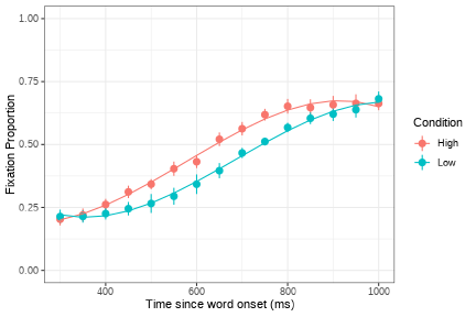
```

![](msmr_lec03_NonLinearLDA_files/figure-html/unnamed-chunk-8-1.png)

---
# The random effects
.pull-left[

```r
head(ranef(m.full)$"Subject")
```

```
##     (Intercept)    poly1      poly2     poly3
## 708  -0.0001522  0.01085 -0.0035635 -0.004929
## 712   0.0110222  0.10693 -0.0093253 -0.036517
## 715   0.0113775  0.11482 -0.0109566 -0.039652
## 720  -0.0020717 -0.01300 -0.0003714  0.003738
## 722   0.0138362  0.16223 -0.0200919 -0.058180
## 725  -0.0178395 -0.20733  0.0253549  0.074204
```
]

.pull-right[

```r
head(ranef(m.full)$"Subject:Condition")
```

```
##          (Intercept)    poly1    poly2    poly3
## 708:High    0.012273 -0.13120 -0.12985  0.01515
## 708:Low    -0.061222  0.17039  0.06228  0.01232
## 712:High    0.021229  0.08290  0.02803  0.02002
## 712:Low    -0.014453  0.04483  0.03255 -0.01730
## 715:High    0.012361  0.05971  0.05517 -0.02500
## 715:Low    -0.008687  0.10599  0.13031 -0.03948
```
]

---
# The random effects

```r
VarCorr(m.full)
```

```
##  Groups            Name        Std.Dev. Corr             
##  Subject:Condition (Intercept) 0.0405                    
##                    poly1       0.1404   -0.43            
##                    poly2       0.1124   -0.33  0.72      
##                    poly3       0.0417    0.13 -0.49 -0.43
##  Subject           (Intercept) 0.0124                    
##                    poly1       0.1195    0.91            
##                    poly2       0.0165   -0.42 -0.76      
##                    poly3       0.0421   -0.85 -0.99  0.83
##  Residual                      0.0438
```

What is being estimated?

* Random variance and covariance
* Unit-level random effects (but constrained to have mean = 0)

**This is why df for parameter estimates are poorly defined in MLM**

---
# Alternative random effects structure

```r
m.left <- lmer(meanFix ~ (poly1+poly2+poly3)*Condition + #fixed effects
 ((poly1+poly2+poly3)*Condition | Subject), #random effects
 data=TargetFix.gca, REML=F)
```

```
## Warning in checkConv(attr(opt, "derivs"), opt$par, ctrl = control$checkConv, :
## Model failed to converge with max|grad| = 0.00339123 (tol = 0.002, component 1)
```

```r
coef(summary(m.left))
```

```
##                      Estimate Std. Error     df   t value  Pr(>|t|)
## (Intercept)         0.4773228    0.01679  9.995 28.428492 6.810e-11
## poly1               0.6385604    0.05146 10.005 12.409428 2.120e-07
## poly2              -0.1095979    0.03719  9.987 -2.946831 1.463e-02
## poly3              -0.0932612    0.02061 10.001 -4.524584 1.100e-03
## ConditionLow       -0.0581122    0.02111  9.994 -2.752959 2.039e-02
## poly1:ConditionLow  0.0003188    0.07481  9.985  0.004262 9.967e-01
## poly2:ConditionLow  0.1635455    0.06278  9.982  2.605219 2.629e-02
## poly3:ConditionLow -0.0020869    0.03332 10.685 -0.062623 9.512e-01
```

---
# Alternative random effects structure

```r
# str(ranef(m.left))
# head(ranef(m.left)$"Subject")
VarCorr(m.left)
```

```
##  Groups   Name               Std.Dev. Corr                                     
##  Subject  (Intercept)        0.0519                                            
##           poly1              0.1569    0.17                                    
##           poly2              0.1095   -0.29  0.03                              
##           poly3              0.0490   -0.28 -0.37  0.63                        
##           ConditionLow       0.0649   -0.89 -0.13  0.49  0.34                  
##           poly1:ConditionLow 0.2286    0.38 -0.46 -0.63  0.10 -0.56            
##           poly2:ConditionLow 0.1890    0.20  0.08 -0.81 -0.22 -0.43  0.74      
##           poly3:ConditionLow 0.0861   -0.08 -0.40 -0.06 -0.47  0.06 -0.27 -0.43
##  Residual                    0.0430
```

This random effect structure makes fewer assumptions:

* Allows unequal variances across conditions
* Allows more flexible covariance structure between random effect terms

---
# Alternative random effects structure requires more parameters

---
# Convergence problems
`Model failed to converge with max|grad| = 0.00930636 (tol = 0.002, component 1)`

## Consider simplifying random effects

**Remove random effects of higher-order terms**

```r
Outcome ~ (poly1+poly2+poly3)*Condition + (poly1+poly2+poly3 | Subject)
Outcome ~ (poly1+poly2+poly3)*Condition + (poly1+poly2 | Subject)
```

**Remove correlation between random effects**

```r
Outcome ~ (poly1+poly2+poly3)*Condition + (1 | Subject) + 
  (0+poly1 | Subject) + (0+poly2 | Subject) + (0+poly3 | Subject)
```

Alternatively: double-pipe

```r
Outcome ~ (poly1+poly2+poly3)*Condition + (poly1+poly2+poly3 || Subject)
```

---
# Participants as fixed vs. random effects
**In general**, participants should be treated as random effects.

This captures the typical assumption of random sampling from some population to which we wish to generalise.

**Pooling**

http://tjmahr.github.io/plotting-partial-pooling-in-mixed-effects-models/

---
# Participants as fixed vs. random effects
**In general**, participants should be treated as random effects.

This captures the typical assumption of random sampling from some population to which we wish to generalise.

**Shrinkage**

http://tjmahr.github.io/plotting-partial-pooling-in-mixed-effects-models/

Another explanation of shrinkage: https://m-clark.github.io/posts/2019-05-14-shrinkage-in-mixed-models/

---
# Participants as fixed vs. random effects
**In general**, participants should be treated as random effects.

This captures the typical assumption of random sampling from some population to which we wish to generalise.

**Exceptions are possible**: e.g., neurological/neuropsychological case studies where the goal is to characterise the pattern of performance for each participant, not generalise to a population.

---
# Key points

.pull-left[
**Modeling non-linear change over time**

* Choose an adequate functional form
    + Polynomials are mathematically nice, but be careful with interpretation and extrapolation
* Random effect structure
    + Keep it maximal, but be ready to deal with convergence problems
    + For within-subject variables: "left" side of pipe (random slopes) is more flexible, but requires more data to estimate; "right" side of pipe (nested) is a good alternative
* Participants as random effects
    + Supports most inferences
    + Partial pooling (aka shrinkage)
    + Some exceptions (e.g., case studies)
]

.pull-right[
<img src="./figs/max_grad_tombstone.jpg" />
]