Data Analysis for Psychology in R 3
Psychology, PPLS
University of Edinburgh
|
Linear Mixed Models (with Elizabeth Pankratz) |
Regression refresher, intro to group-structured data |
| Modelling group-structured data using random effects | |
| Interpreting LMMs and building maximal models | |
| Troubleshooting model fit, checking assumptions + diagnostics | |
| LMMs: Practice analysis | |
|
Factor Analysis working with multi-item measures (with Josiah King) |
measurement and dimensionality |
| exploring underlying constructs (EFA) | |
| testing theoretical models (CFA) | |
| reliability and validity | |
| recap & exam prep |
Labs:
Lecture consolidation:

for our purposes:
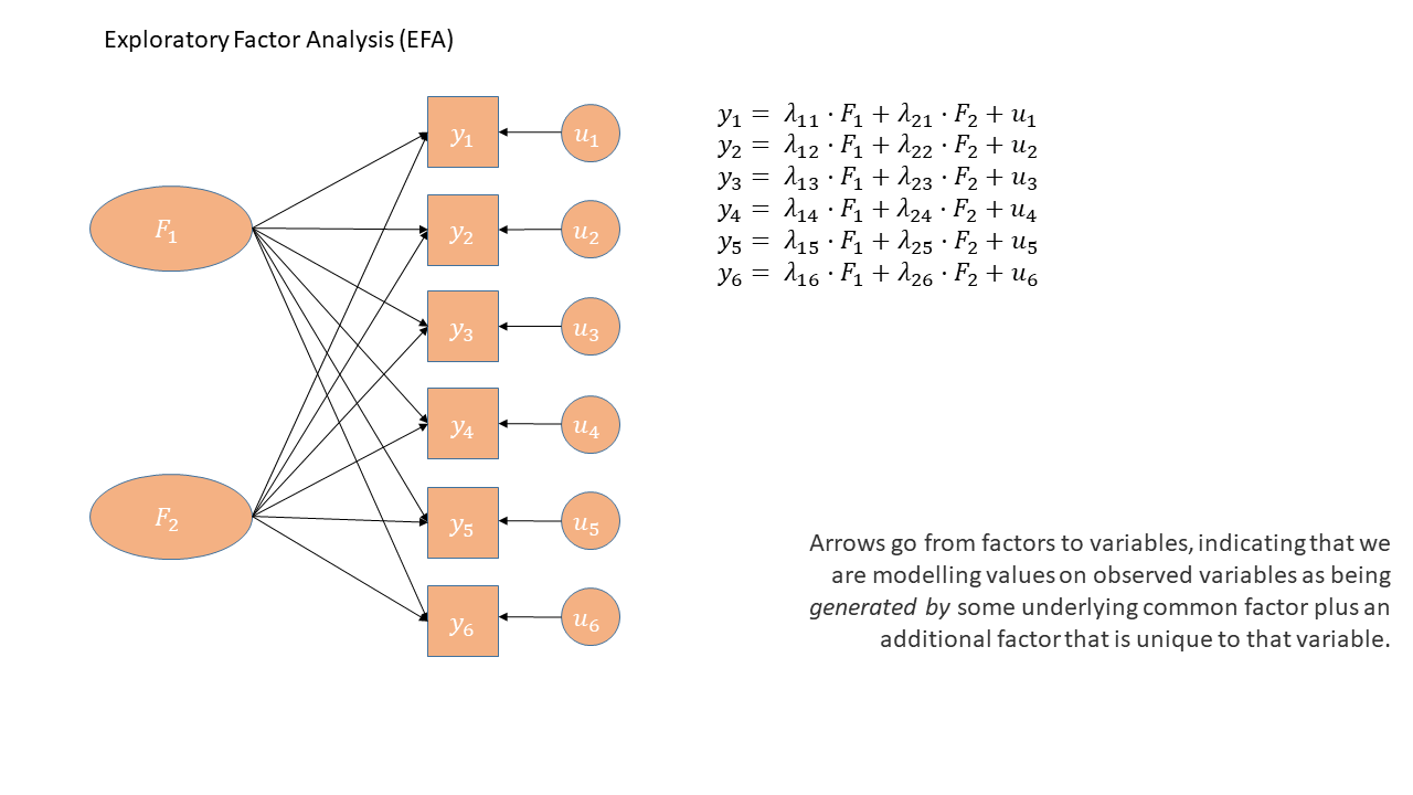
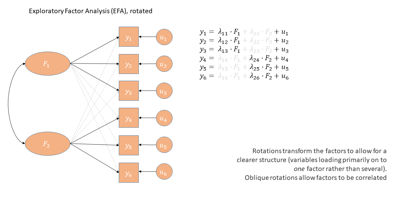
item ~ factor(all of these things can be relaxed with more advanced methods)
“latent variable analysis”
general modelling framework that estimates models that may include latent variables
Previously:
lm(formula, data)glm(formula, data)lmer(formula, data)With lavaan:
Specify model formula in quotation marks:
mymod <- "................"
Estimate1 formula with a fitting function such as:
mymod.est <- cfa(mymod, data)
| Formula type | Operator | Mnemonic |
|---|---|---|
| latent variable definition | =~ |
“is measured by” |
| (residual) (co)variance | ~~ |
“covaries with” |
| regression | ~ |
“is regressed on” |

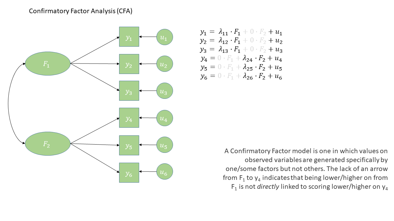
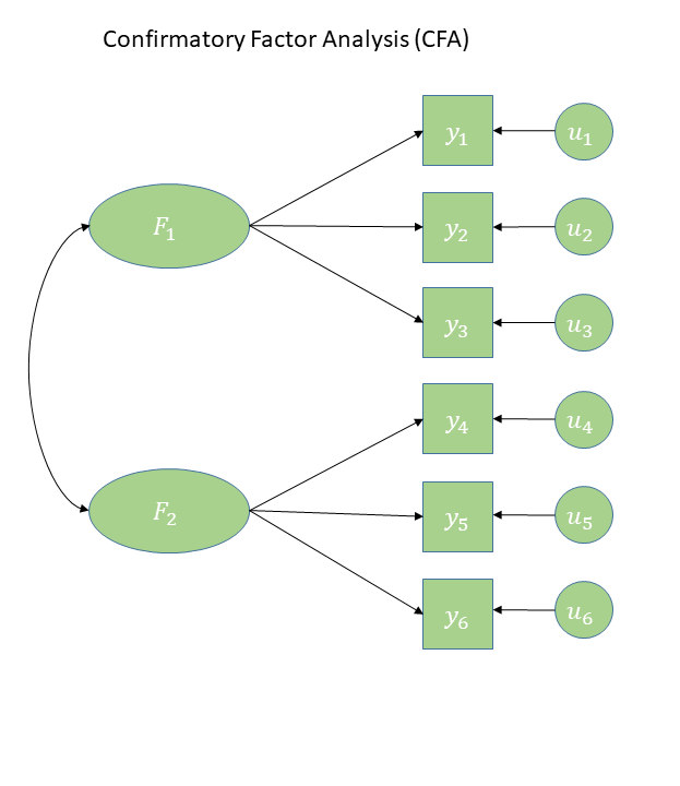
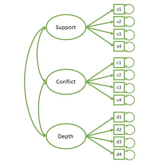
F1 =~ y1 + y2 + y3
F2 =~ y4 + y5 + y6
F1 ~~ F2

| var | wording |
|---|---|
| s1 | To what extent could you turn to this person for advice about problems? |
| s2 | To what extent could you count on this person for help with a problem? |
| s3 | To what extent can you really count on this person to distract you from your worries when you feel under stress? |
| s4 | To what extent can you count on this person to listen to you when you are very angry at someone else? |
| c1 | How often do you have to work hard to avoid conflict with this person? |
| c2 | How much do you argue with this person? |
| c3 | How much would you like this person to change? |
| c4 | How often does this person make you feel angry? |
| d1 | How positive a role does this person play in your life? |
| d2 | How significant is this relationship in your life? |
| d3 | How close will your relationship be with this person in 10 years? |
| d4 | How much would you miss this person if the two of you could not see or talk with each other for a month? |
s2 d4 c3 c4 d1 c2 s1 s4 d2 c1 s3 d3
1 4 4 5 5 5 4 3 3 2 3 5 5
2 3 5 4 4 2 4 4 5 2 4 4 4
3 4 5 4 5 4 2 5 3 6 2 4 5
4 3 6 4 3 5 3 3 4 4 2 5 5
5 6 7 1 2 4 2 7 7 4 1 7 5
6 3 5 5 4 4 3 5 4 3 3 5 5
lavaan 0.7-2 ended normally after 19 iterations
Estimator ML
Optimization method NLMINB
Number of model parameters 27
Number of observations 374
Model Test User Model:
Test statistic 81.100
Degrees of freedom 51
P-value (Chi-square) 0.005
Parameter Estimates:
Standard errors Standard
Information Expected
Information saturated (h1) model Structured
Latent Variables:
Estimate Std.Err z-value P(>|z|) Std.lv Std.all
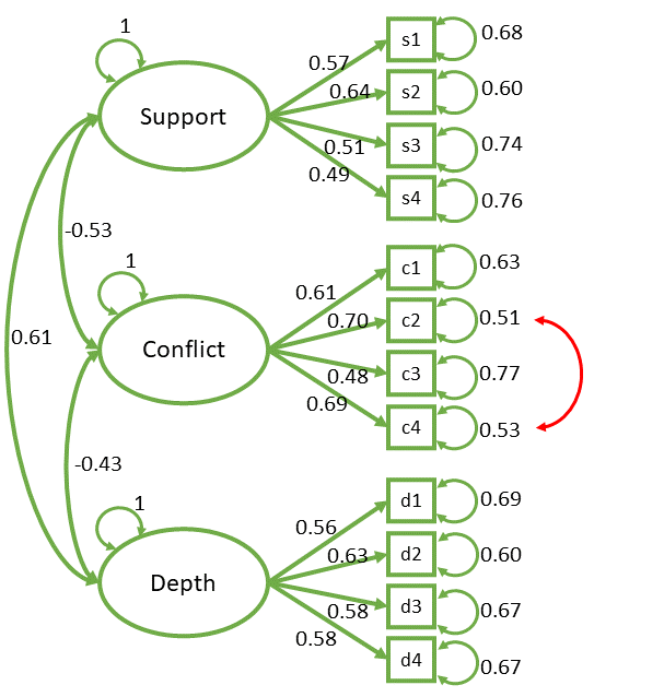
support =~
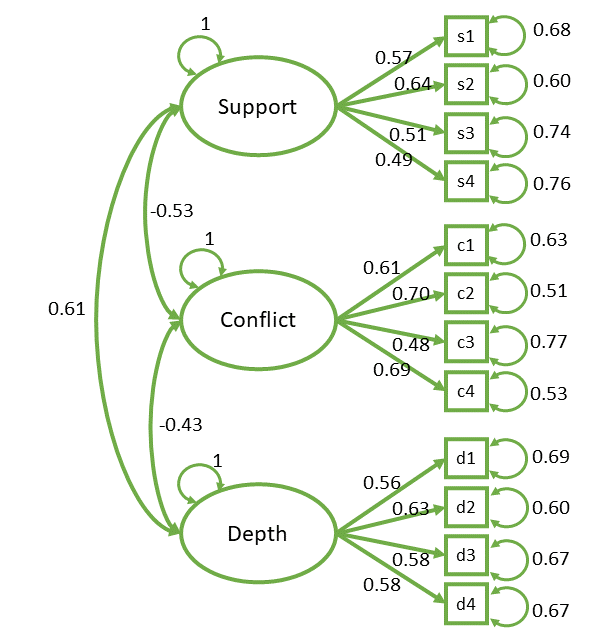
s1 0.601 0.062 9.765 0.000 0.601 0.567
s2 0.707 0.064 11.010 0.000 0.707 0.636
s3 0.642 0.074 8.676 0.000 0.642 0.508
s4 0.608 0.072 8.407 0.000 0.608 0.493
conflict =~
c1 0.860 0.077 11.102 0.000 0.860 0.608
c2 0.810 0.063 12.909 0.000 0.810 0.698
c3 0.614 0.072 8.532 0.000 0.614 0.481
c4 0.808 0.064 12.673 0.000 0.808 0.686
depth =~
d1 0.617 0.063 9.759 0.000 0.617 0.559
d2 0.770 0.069 11.175 0.000 0.770 0.633
d3 0.621 0.061 10.119 0.000 0.621 0.578
d4 0.634 0.062 10.143 0.000 0.634 0.579
Covariances:
Estimate Std.Err z-value P(>|z|) Std.lv Std.all
support ~~
conflict -0.530 0.063 -8.473 0.000 -0.530 -0.530
depth 0.613 0.062 9.956 0.000 0.613 0.613
conflict ~~
depth -0.425 0.065 -6.551 0.000 -0.425 -0.425
Variances:
Estimate Std.Err z-value P(>|z|) Std.lv Std.all
.s1 0.763 0.070 10.860 0.000 0.763 0.679
.s2 0.738 0.077 9.626 0.000 0.738 0.596
.s3 1.188 0.102 11.625 0.000 1.188 0.742
.s4 1.151 0.098 11.781 0.000 1.151 0.757
.c1 1.259 0.116 10.893 0.000 1.259 0.630
.c2 0.692 0.076 9.128 0.000 0.692 0.513
.c3 1.251 0.102 12.276 0.000 1.251 0.768
.c4 0.735 0.078 9.409 0.000 0.735 0.529
.d1 0.839 0.075 11.146 0.000 0.839 0.688
.d2 0.885 0.089 9.923 0.000 0.885 0.599
.d3 0.771 0.071 10.880 0.000 0.771 0.666
.d4 0.797 0.073 10.861 0.000 0.797 0.665
support 1.000 1.000 1.000
conflict 1.000 1.000 1.000
depth 1.000 1.000 1.000
on what scale are our latent variables?
on what scale do we want our estimated parameters?
latent variables are unobserved abstractions.
they have no intrinsic numeric scale, so we need to fix it to something
Options (when estimating):
fix latent variables to unit variance (\(sd = 1\))
cfa(model, data)
fix loading of first item to 1 (thereby fixing it to the same scale as the first item)
cfa(model, data, std.lv = TRUE)
None of this changes the model. The fit will be identical
Options:
keep variables in original units, keep latent variables on whatever scale they were fitted.
parameterestimates(model)
partially standardised - rescale only the latent variables to unit variance (\(sd = 1\)). observed variables stay in their original units.
completely standardised - rescale both observed variables and latent variables to unit variance (\(sd = 1\)). We get standardised factor loadings (like EFA) and factor covariances become correlations.
standardizedSolution(model)
Everything, all at once: summary(model, std = TRUE)
provides Estimate, std.lv, and std.all
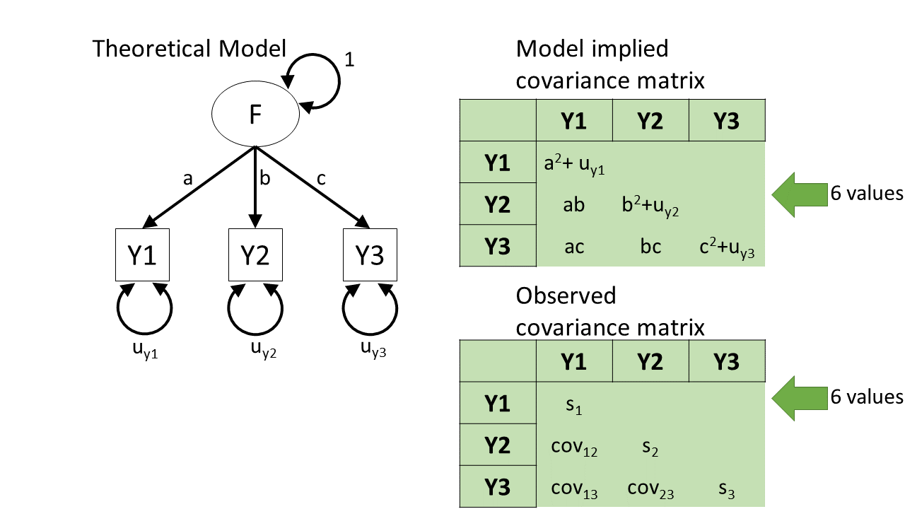
“how well does my model reproduce my outcome?”
\[ \begin{align} \text{outcome} &= \text{model} &+ \text{error} \\ \quad \\ \text{observed variable} & = \text{coefficients and predictor variables} &+ \text{error} \\ \quad \\ \text{observed variable} & = \text{model predicted values} &+ \text{error} \\ \end{align} \]
\[ \begin{align} \text{outcome} &= \text{model} &+ \quad \text{error} \\ \quad \\ \text{observed correlation matrix} & = \begin{aligned}[c] &\text{factor loadings} \\ &\text{(maybe rotated)} \end{aligned} &+\quad \text{unique variance} \\ \end{align} \]
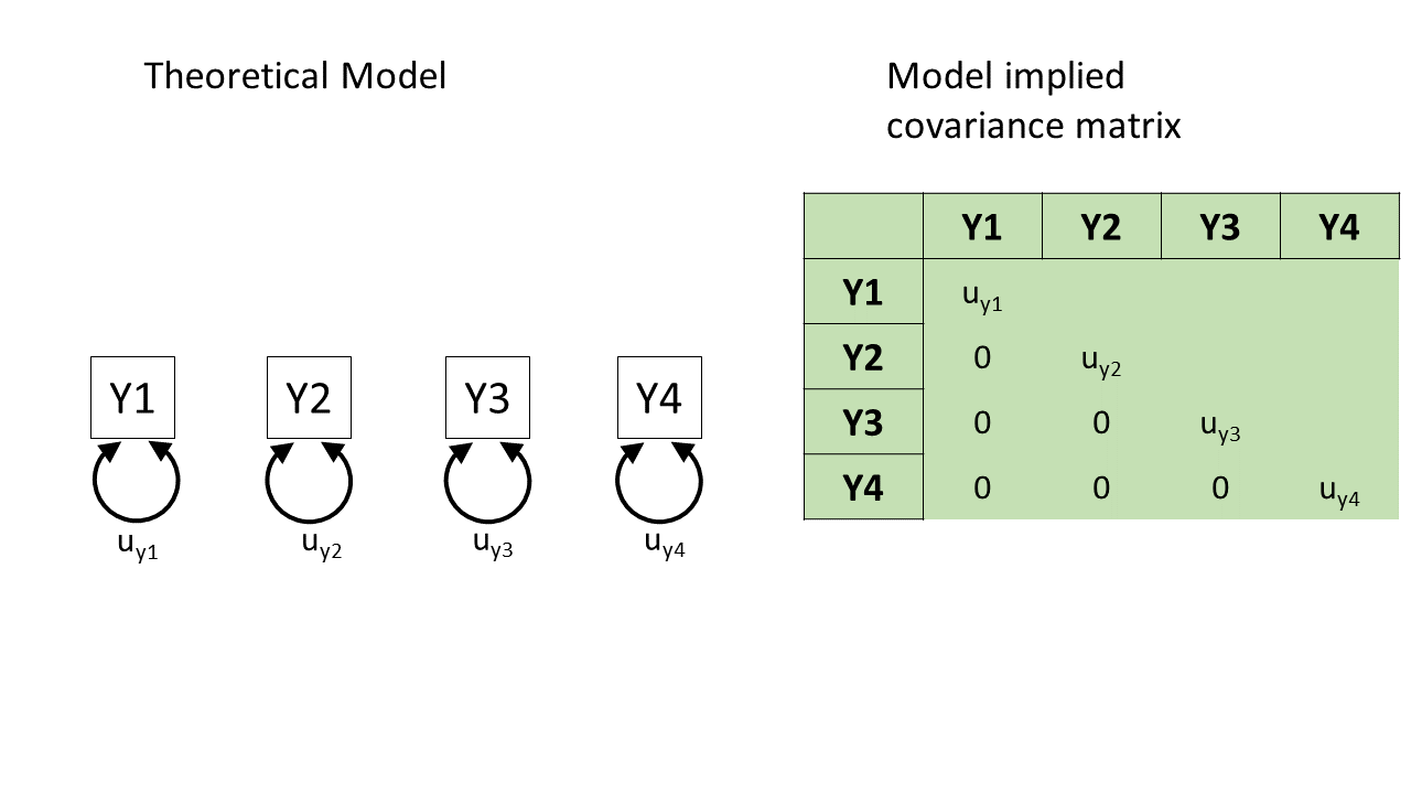
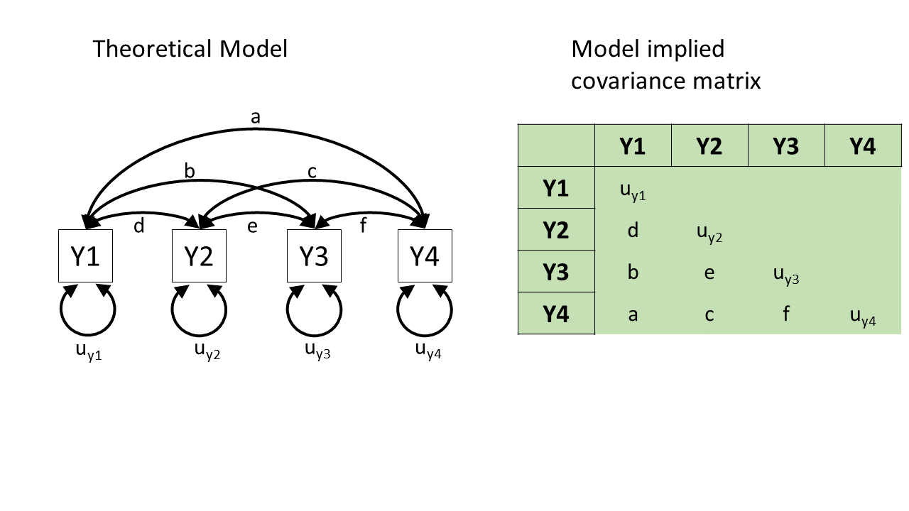
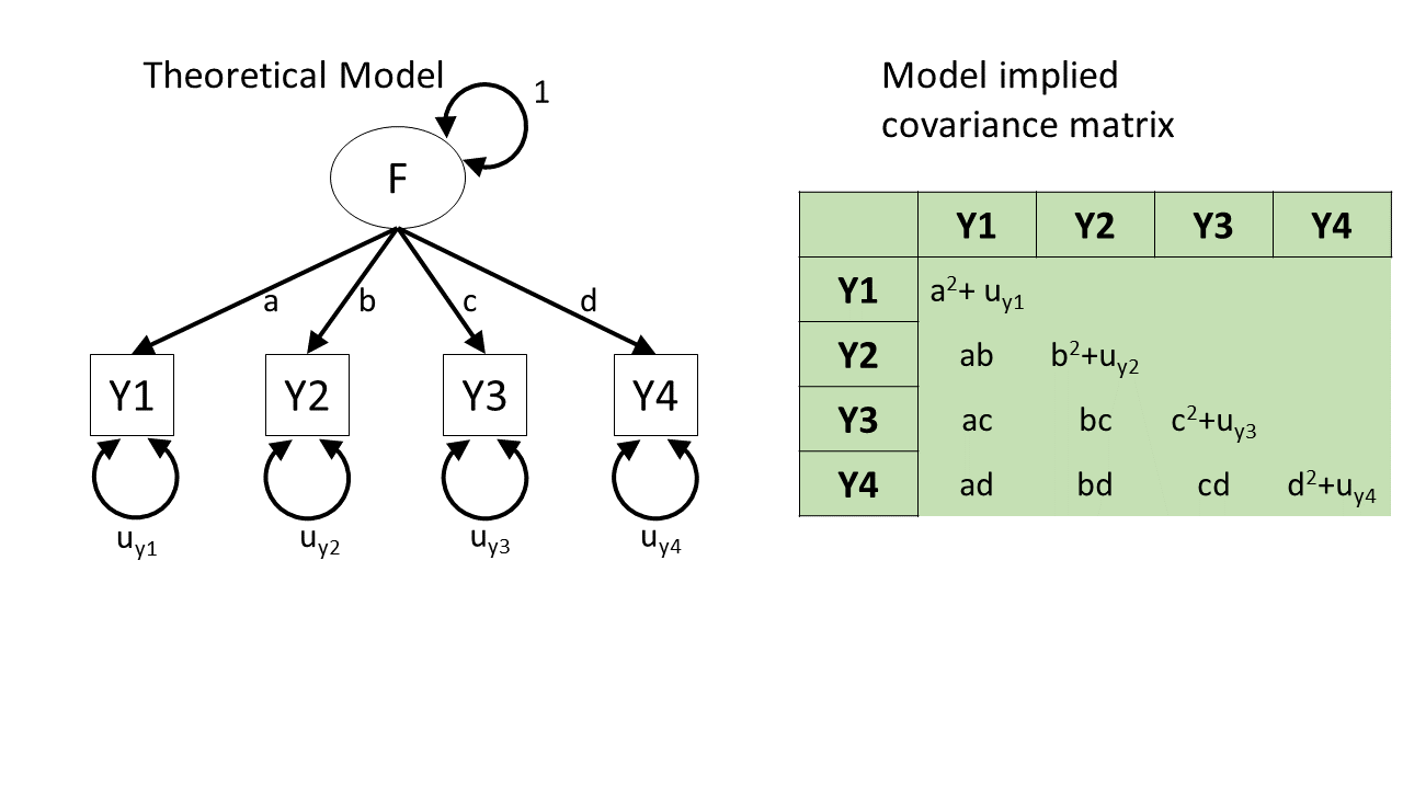
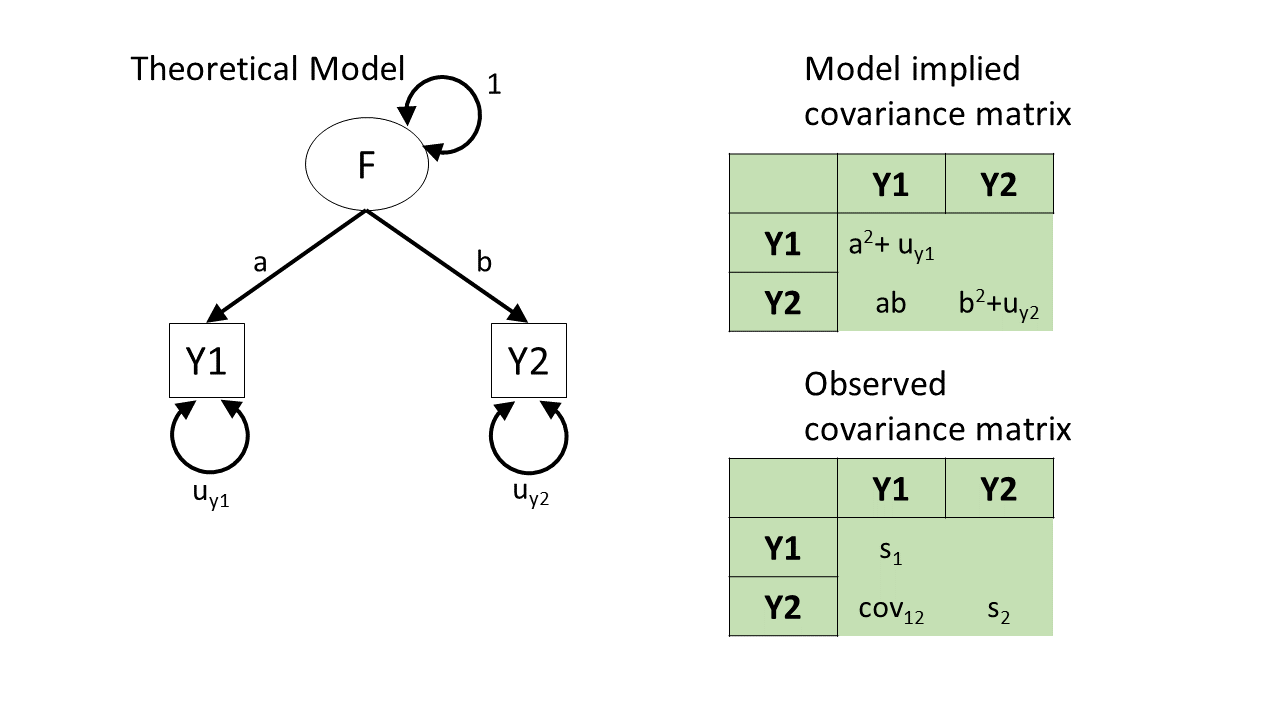
\[ \begin{align} \text{outcome} &= \text{model} &+ \text{error} \\ \quad \\ \text{observed covariance matrix} & = \text{model parameters} &+ \text{unique variance} \\ \quad \\ &... \\ &... \\ &... \\ \quad \\ \text{observed covariance matrix} & = \text{model implied covariance matrix} &+ \text{unique variance} \\ \end{align} \]
Conceptually:
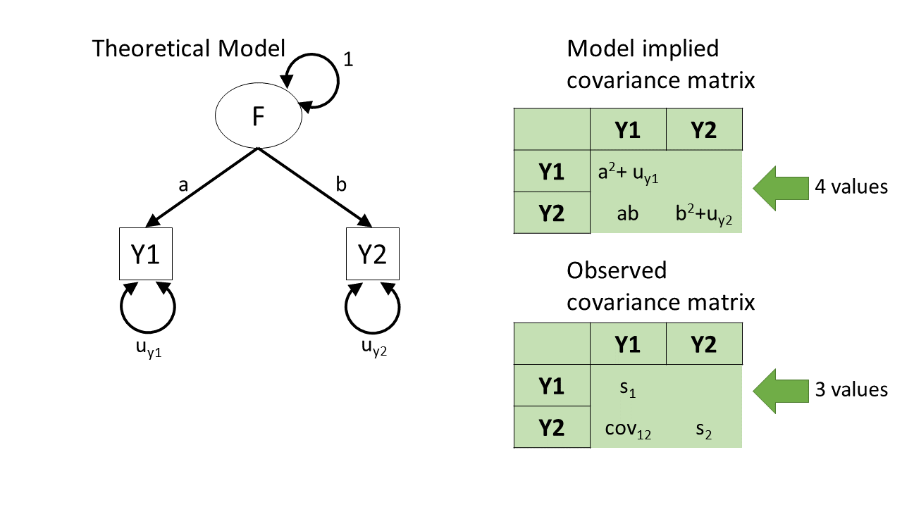
To measure ‘model fit’ we need to observe more things than we estimate
how many “knowns”?
how many values in our covariance matrix?
for \(k\) variables this is \(\frac{k(k+1)}{2}\)
how many “unknowns”?
degrees of freedom = knowns - unknowns
how many “knowns”?
s2 d4 c3 c4 d1 c2 s1 s4 d2 c1 s3 d3
s2 1.24 0.32 -0.26 -0.24 0.22 -0.21 0.46 0.39 0.39 -0.46 0.44 0.31
d4 0.32 1.20 -0.19 -0.10 0.39 -0.20 0.20 0.29 0.47 -0.40 0.24 0.41
c3 -0.26 -0.19 1.63 0.41 -0.24 0.43 -0.31 -0.32 -0.34 0.68 -0.24 -0.29
c4 -0.24 -0.10 0.41 1.39 -0.15 0.78 -0.24 -0.24 -0.16 0.62 -0.29 -0.14
d1 0.22 0.39 -0.24 -0.15 1.22 -0.22 0.19 0.16 0.51 -0.42 0.24 0.38
c2 -0.21 -0.20 0.43 0.78 -0.22 1.35 -0.18 -0.18 -0.17 0.62 -0.26 -0.20
s1 0.46 0.20 -0.31 -0.24 0.19 -0.18 1.13 0.36 0.28 -0.38 0.37 0.20
s4 0.39 0.29 -0.32 -0.24 0.16 -0.18 0.36 1.53 0.29 -0.45 0.45 0.24
d2 0.39 0.47 -0.34 -0.16 0.51 -0.17 0.28 0.29 1.48 -0.37 0.32 0.46
c1 -0.46 -0.40 0.68 0.62 -0.42 0.62 -0.38 -0.45 -0.37 2.00 -0.30 -0.32
s3 0.44 0.24 -0.24 -0.29 0.24 -0.26 0.37 0.45 0.32 -0.30 1.61 0.23
d3 0.31 0.41 -0.29 -0.14 0.38 -0.20 0.20 0.24 0.46 -0.32 0.23 1.16
how many “unknowns”?
how many “knowns”?
78 variances and covariances
how many “unknowns”?
27 estimated parameters
Pretty much all based on:
\[
\begin{align}
\text{observed covariance matrix}\,\,\, vs \,\,\, \text{model implied covariance matrix}\\
\end{align}
\]
they typically also incorporate degrees of freedom (this represents model complexity/parsimony)
there are loooooooaddds of different metrics…
“absolute fit”
“how far from perfect fit?”
smaller is better
| fit index | common threshold |
|---|---|
| RMSEA | <0.05 |
| SRMR | <0.05/<0.08 |
“incremental fit”
“how much better than a null model1?”
bigger is better
| fit index | common threshold |
|---|---|
| TLI | >0.95 |
| CFI | >0.95 |
In R:
fitmeasures(mymod.est)[c("rmsea","srmr","cfi","tli")]
rmsea srmr cfi tli
0.0397 0.0467 0.9619 0.9508
“how much better would my model fit if we included parameter XXX?”
but..
lhs, op, rhs = the parametermi = change in fitepc, sepc.lv, sepc.all, sepc.nox = expected value of parameter (under various forms of standardisation) lhs op rhs mi epc sepc.lv sepc.all sepc.nox
101 c2 ~~ c4 50.316 0.561 0.561 0.787 0.787
51 depth =~ c1 15.882 -0.378 -0.378 -0.267 -0.267
31 support =~ c1 14.774 -0.417 -0.417 -0.295 -0.295
54 depth =~ c4 12.504 0.282 0.282 0.239 0.239
32 support =~ c2 9.875 0.287 0.287 0.247 0.247
94 c1 ~~ c3 8.577 0.237 0.237 0.189 0.189
93 c1 ~~ c2 8.101 -0.241 -0.241 -0.258 -0.258
95 c1 ~~ c4 7.628 -0.234 -0.234 -0.243 -0.243
53 depth =~ c3 6.143 -0.216 -0.216 -0.170 -0.170
106 c3 ~~ c4 6.027 -0.170 -0.170 -0.177 -0.177
33 support =~ c3 5.216 -0.227 -0.227 -0.178 -0.178
100 c2 ~~ c3 3.797 -0.134 -0.134 -0.144 -0.144
34 support =~ c4 3.637 0.176 0.176 0.149 0.149
96 c1 ~~ d1 3.523 -0.116 -0.116 -0.113 -0.113
99 c1 ~~ d4 3.320 -0.111 -0.111 -0.111 -0.111
114 c4 ~~ d4 3.179 0.087 0.087 0.114 0.114
52 depth =~ c2 2.985 0.136 0.136 0.117 0.117
68 s2 ~~ c1 2.819 -0.103 -0.103 -0.107 -0.107
108 c3 ~~ d2 2.611 -0.102 -0.102 -0.097 -0.097
85 s4 ~~ c1 2.474 -0.112 -0.112 -0.093 -0.093
103 c2 ~~ d2 2.117 0.076 0.076 0.097 0.097
59 s1 ~~ c2 2.114 0.069 0.069 0.095 0.095
60 s1 ~~ c3 1.940 -0.079 -0.079 -0.081 -0.081
86 s4 ~~ c2 1.895 0.078 0.078 0.087 0.087
77 s3 ~~ c1 1.835 0.099 0.099 0.081 0.081
109 c3 ~~ d3 1.748 -0.076 -0.076 -0.077 -0.077
67 s2 ~~ s4 1.658 -0.089 -0.089 -0.096 -0.096
69 s2 ~~ c2 1.603 0.062 0.062 0.086 0.086
89 s4 ~~ d1 1.592 -0.073 -0.073 -0.074 -0.074
55 s1 ~~ s2 1.525 0.078 0.078 0.103 0.103
35 support =~ d1 1.494 -0.127 -0.127 -0.115 -0.115
72 s2 ~~ d1 1.414 -0.060 -0.060 -0.076 -0.076
47 depth =~ s1 1.403 -0.122 -0.122 -0.115 -0.115
48 depth =~ s2 1.326 0.131 0.131 0.117 0.117
87 s4 ~~ c3 1.326 -0.078 -0.078 -0.065 -0.065
76 s3 ~~ s4 1.244 0.083 0.083 0.071 0.071
92 s4 ~~ d4 1.145 0.061 0.061 0.064 0.064
115 d1 ~~ d2 0.991 0.067 0.067 0.078 0.078
80 s3 ~~ c4 0.971 -0.058 -0.058 -0.062 -0.062
111 c4 ~~ d1 0.853 0.046 0.046 0.059 0.059
73 s2 ~~ d2 0.779 0.048 0.048 0.059 0.059
75 s2 ~~ d4 0.743 0.043 0.043 0.056 0.056
110 c3 ~~ d4 0.682 0.048 0.048 0.048 0.048
65 s1 ~~ d4 0.678 -0.039 -0.039 -0.051 -0.051
44 conflict =~ d2 0.667 0.069 0.069 0.057 0.057
58 s1 ~~ c1 0.660 -0.049 -0.049 -0.050 -0.050
71 s2 ~~ c4 0.616 0.039 0.039 0.053 0.053
113 c4 ~~ d3 0.574 0.036 0.036 0.048 0.048
43 conflict =~ d1 0.558 -0.056 -0.056 -0.051 -0.051
74 s2 ~~ d3 0.541 0.036 0.036 0.047 0.047
40 conflict =~ s2 0.521 0.067 0.067 0.060 0.060
112 c4 ~~ d2 0.493 0.037 0.037 0.046 0.046
64 s1 ~~ d3 0.371 -0.029 -0.029 -0.037 -0.037
78 s3 ~~ c2 0.370 -0.035 -0.035 -0.039 -0.039
118 d2 ~~ d3 0.360 -0.040 -0.040 -0.048 -0.048
119 d2 ~~ d4 0.340 -0.039 -0.039 -0.047 -0.047
102 c2 ~~ d1 0.304 -0.027 -0.027 -0.035 -0.035
36 support =~ d2 0.304 0.065 0.065 0.054 0.054
42 conflict =~ s4 0.285 -0.052 -0.052 -0.042 -0.042
66 s2 ~~ s3 0.263 -0.037 -0.037 -0.039 -0.039
120 d3 ~~ d4 0.259 0.029 0.029 0.037 0.037
56 s1 ~~ s3 0.190 -0.028 -0.028 -0.030 -0.030
84 s3 ~~ d4 0.175 -0.024 -0.024 -0.025 -0.025
38 support =~ d4 0.173 0.043 0.043 0.039 0.039
105 c2 ~~ d4 0.166 -0.020 -0.020 -0.026 -0.026
83 s3 ~~ d3 0.158 -0.023 -0.023 -0.024 -0.024
79 s3 ~~ c3 0.152 0.027 0.027 0.022 0.022
81 s3 ~~ d1 0.147 0.023 0.023 0.023 0.023
45 conflict =~ d3 0.104 -0.024 -0.024 -0.022 -0.022
70 s2 ~~ c3 0.085 0.017 0.017 0.018 0.018
104 c2 ~~ d3 0.074 -0.013 -0.013 -0.018 -0.018
82 s3 ~~ d2 0.042 0.013 0.013 0.013 0.013
91 s4 ~~ d3 0.040 0.011 0.011 0.012 0.012
61 s1 ~~ c4 0.039 -0.010 -0.010 -0.013 -0.013
37 support =~ d3 0.034 0.019 0.019 0.017 0.017
117 d1 ~~ d4 0.033 -0.011 -0.011 -0.013 -0.013
62 s1 ~~ d1 0.031 -0.009 -0.009 -0.011 -0.011
41 conflict =~ s3 0.030 -0.017 -0.017 -0.014 -0.014
46 conflict =~ d4 0.027 0.012 0.012 0.011 0.011
39 conflict =~ s1 0.023 -0.013 -0.013 -0.012 -0.012
49 depth =~ s3 0.021 -0.017 -0.017 -0.014 -0.014
88 s4 ~~ c4 0.019 0.008 0.008 0.009 0.009
63 s1 ~~ d2 0.017 0.007 0.007 0.008 0.008
116 d1 ~~ d3 0.014 -0.007 -0.007 -0.008 -0.008
107 c3 ~~ d1 0.011 -0.006 -0.006 -0.006 -0.006
50 depth =~ s4 0.009 0.011 0.011 0.009 0.009
98 c1 ~~ d3 0.005 0.004 0.004 0.004 0.004
97 c1 ~~ d2 0.004 -0.004 -0.004 -0.004 -0.004
57 s1 ~~ s4 0.003 -0.003 -0.003 -0.004 -0.004
90 s4 ~~ d2 0.002 -0.003 -0.003 -0.003 -0.003
| var | wording |
|---|---|
| s1 | To what extent could you turn to this person for advice about problems? |
| s2 | To what extent could you count on this person for help with a problem? |
| s3 | To what extent can you really count on this person to distract you from your worries when you feel under stress? |
| s4 | To what extent can you count on this person to listen to you when you are very angry at someone else? |
| c1 | How often do you have to work hard to avoid conflict with this person? |
| c2 | How much do you argue with this person? |
| c3 | How much would you like this person to change? |
| c4 | How often does this person make you feel angry? |
| d1 | How positive a role does this person play in your life? |
| d2 | How significant is this relationship in your life? |
| d3 | How close will your relationship be with this person in 10 years? |
| d4 | How much would you miss this person if the two of you could not see or talk with each other for a month? |
Less contentious uses:
More contentious uses:
adding cross-loadings (could argue that an item loading on two factors is not a clean indicator, and so should be removed)
residual covariances for items on different factors - harder to defend
changing paths between the latent variables - very definitely changing your theory!
re-specifying a model is no longer confirmatory
it is exploratory again!
gaahhhh
there are so many parts to these models that often the “interpretation” such as it is, will boil down to:
And then the bit we might be more interested in, things like: