Exploratory Factor Analysis (EFA)

Data Analysis for Psychology in R 3

Josiah King - josiah.king@ed.ac.uk

Psychology, PPLS

University of Edinburgh

Course Overview


Linear Mixed Models
(with Elizabeth Pankratz)
Regression refresher, intro to group-structured data
Modelling group-structured data using random effects
Interpreting LMMs and building maximal models
Troubleshooting model fit, checking assumptions + diagnostics
LMMs: Practice analysis
Factor Analysis
working with multi-item measures
(with Josiah King)
measurement and dimensionality
exploring underlying constructs (EFA)
testing theoretical models (CFA)
reliability and validity
recap & exam prep

Week 7 TR;DL

  1. measurement is hard, especially in psych
  2. multi-item measurement tools mean we have lots of variables capturing the same thing (lots of “dimensions”)
  3. our goal in the second half of DAPR3 is to explore ways of expressing a lot of the same information using fewer variables (“dimensionality reduction”)
  4. one way to reduce dimensionality is to take a scale score (i.e., mean or sum of all individual scores)
    • this assumes each item is equally representative of our construct
  5. another way is PCA:
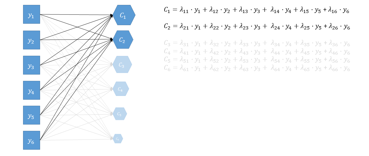
    • for \(k\) variable, finds \(k\) new dimensions (“components”) that:
      • are a weighted sum of original variables:
      • sequentially capture variability in the data
      • are orthogonal (uncorrelated) to one another
        • we then reduce by taking the first \(k\) components
  6. a constant reminder: getting some numbers is not the same thing as measurement

Today

  • from reduction to measurement models (from PCA to EFA)
  • Why EFA?
  • How (broadly) EFA works
  • “Rotations” & Simple Structures
  • Evaluating Factor Solutions

This Week

Conceptual overview

What… is your quest?

PCA
  • Why are your variables correlated?
    • Agnostic/don’t care


  • Goals:
    • Reduce reduce reduce!
    • get some scores
EFA
  • Why are your variables correlated?
    • There exist some number of underlying “causes” of the correlations


  • Goals:
    • learn about/model the underlying cause(s)
    • (optional) estimate some scores

What… are your new dimensions?

PCA: Components
  • a weighted composite of the variables.
    • “a little bit of column A, a little bit of column B”
  • nothing more.
EFA: Factors
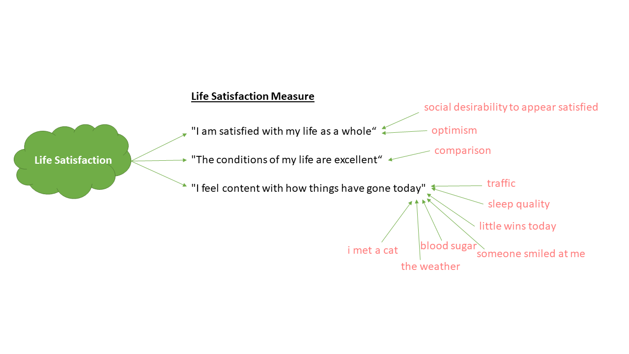
  • theorized common cause of responses to a set of variables

  • something that explains correlations between measured variables

  • assumed to be real (unobservable) things in the world

PCA

  • portion up all/any variance into distinct buckets
  • keep the biggest bucket(s)

EFA

  • separate out common variance (shared across items) from unique variance
  • keep the meaningful underlying drivers of shared variance
Sources of variance

\[ \begin{equation} \text{Var}(\text{total}) = \text{Var}(\text{common}) + \underbrace{\text{Var}(\text{specific}) + \text{Var}(\text{error})}_{\text{unique variance}} \end{equation} \]


common variance (co)variance shared across items true and shared
specific variance variance specific to an item that is not shared with any other items true and unique
error variance variance due to measurement error not ‘true’, unique

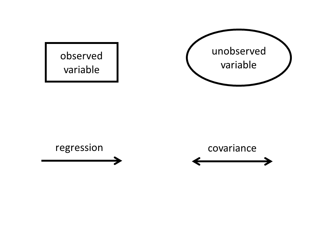
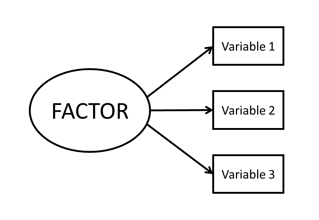
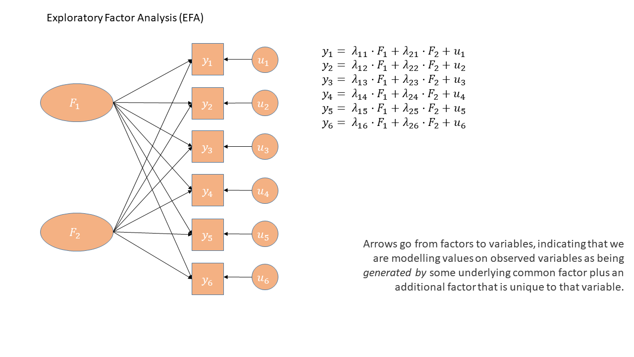
thinking in diagrams

thinking in diagrams (2)
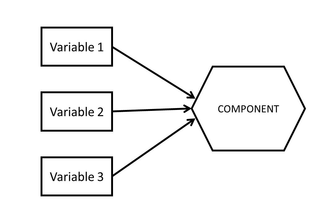

PCA

EFA

directions & magnitudes in PCA

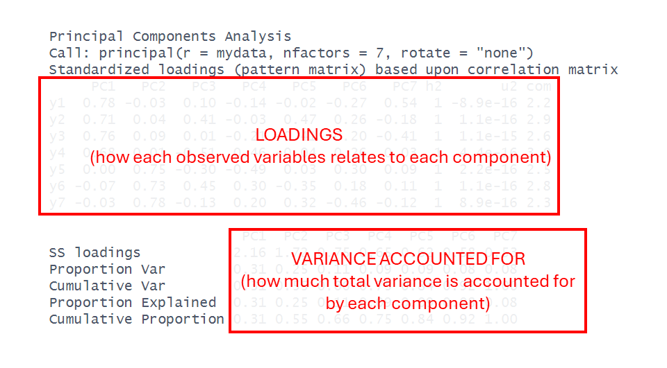
  • Last week was mainly about % variance accounted for by each principal component

  • We didn’t look at the loadings much..

directions & magnitudes in EFA

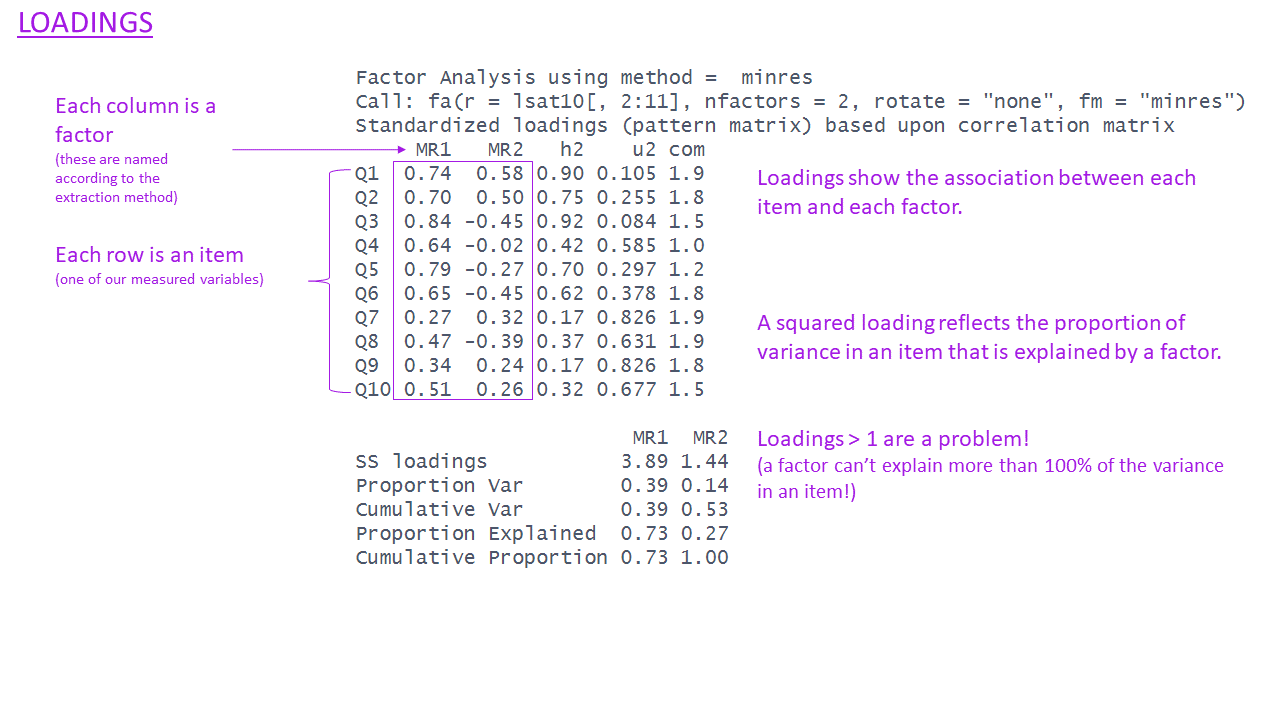
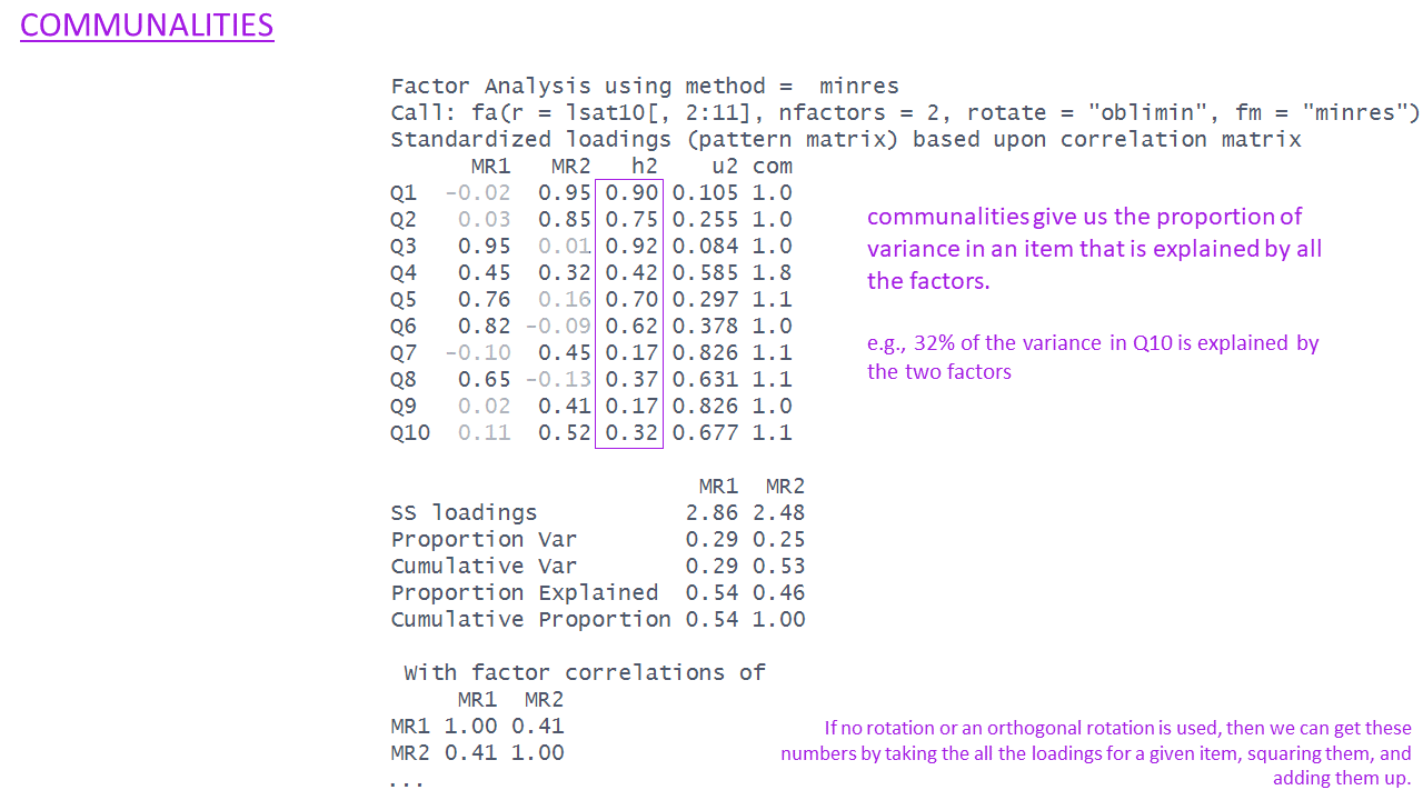
  • In EFA we still get “loadings” and “variance accounted for”

  • The patterns of loadings will help us understand what the latent factors actually are.
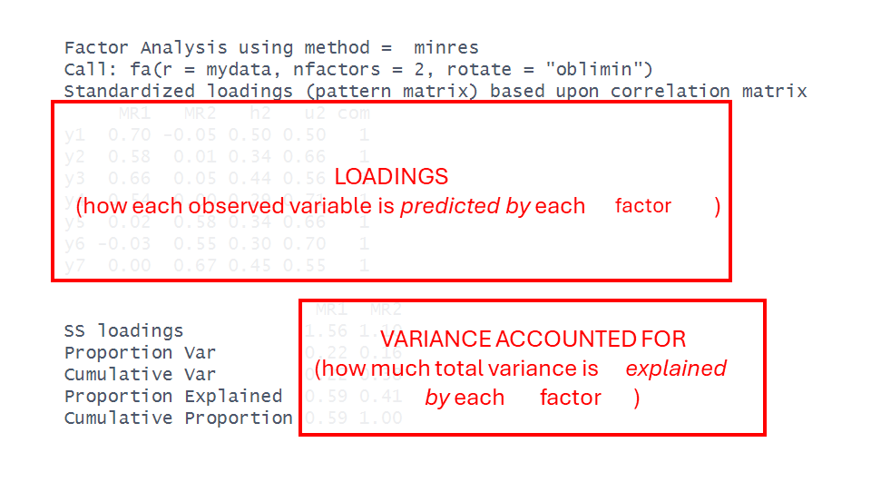
EFA: modelling correlations

  • We have some observed variables that are correlated

  • Latent factor(s) are unobservable variables that explain the patterns of correlations.

  • Idea is that the correlations between items after removing the effect of the Factor are zero

id True_LS Q1 Q2 Q3
P001 44.5 40 50 20
P002 36.9 30 40 70
P003 43.3 77 72 56
P004 39.7 65 60 90
P005 30.6 57 56 39
P006 44.7 41 41 26

\[ \begin{align} \rho(Q_{1},Q_{2}\, |\, \color{grey}{\textrm{True_LS}})=0 \\ \rho(Q_{1},Q_{3}\, |\, \color{grey}{\textrm{True_LS}})=0 \\ \rho(Q_{2},Q_{3}\, |\, \color{grey}{\textrm{True_LS}})=0 \\ \end{align} \]

EFA: modelling correlations

\(\begin{align}\text{Outcome} \quad\quad\quad\quad\quad &=& \quad\quad\text{Model} \quad\quad\quad\quad\quad&+&\quad\quad\text{Error} \\\end{align}\)

\(\begin{align}\text{Correlation matrix} \quad &=& \quad \begin{aligned}[c] &\text{How each variable} \\ &\text{reflects the shared} \\ &\text{factor(s)} \end{aligned} \quad&+&\quad \begin{aligned}[c] &\text{How each variable} \\ &\text{uniquely varies} \end{aligned} \\ \end{align}\)

\(\begin{align} \text{Correlation matrix} \quad &=& \quad\text{Factor loadings} \quad\quad\quad&+&\quad \text{Unique variances} \\ \end{align}\)

EFA: modelling correlations

\[ \begin{align} \text{Outcome} &= \quad\quad\quad\text{Model} &&+ \text{Error} \quad\quad\quad\quad\quad \\ \quad \\ \text{Correlation Matrix} &= \quad\quad\quad\begin{aligned}[c] &\text{How each variable} \\ &\text{reflects the shared} \\ &\text{factor(s)} \end{aligned} &&+ \begin{aligned}[c] &\text{How each variable} \\ &\text{is unique} \end{aligned} \\ \quad \\ \text{Correlation matrix} &= \quad\quad\quad\text{Factor loadings} &&+ \text{Unique variances} \quad\quad\quad\quad\quad \\ \quad \\ \quad \\ \mathbf{\Sigma} &= \quad\quad\quad\mathbf{\Lambda}\mathbf{\Lambda'} &&+ \mathbf{\Psi} \quad\quad\quad\quad\quad\quad \\ \quad \\ \begin{bmatrix} 1 & 0.53 & 0.57 & 0.57 \\ 0.53 & 1 & 0.54 & 0.56 \\ 0.57 & 0.54 & 1 & 0.56 \\ 0.57 & 0.56 & 0.56 & 1 \\ \end{bmatrix} &= \begin{bmatrix} 0.747 \\ 0.725 \\ 0.746 \\ 0.764 \\ \end{bmatrix} \begin{bmatrix} 0.747 & 0.725 & 0.746 & 0.764 \\ \end{bmatrix} &&+ \begin{bmatrix} 0.44 & 0 & 0 & 0 \\ 0 & 0.47 & 0 & 0 \\ 0 & 0 & 0.44 & 0 \\ 0 & 0 & 0 & 0.42 \\ \end{bmatrix} \\ \quad \\ \begin{bmatrix} 1 & 0.53 & 0.57 & 0.57 \\ 0.53 & 1 & 0.54 & 0.56 \\ 0.57 & 0.54 & 1 & 0.56 \\ 0.57 & 0.56 & 0.56 & 1 \\ \end{bmatrix} &= \begin{bmatrix} 0.56 & 0.54 & 0.56 & 0.57 \\ 0.54 & 0.53 & 0.54 & 0.55 \\ 0.56 & 0.54 & 0.56 & 0.57 \\ 0.57 & 0.55 & 0.57 & 0.58 \\ \end{bmatrix} &&+ \begin{bmatrix} 0.44 & 0 & 0 & 0 \\ 0 & 0.47 & 0 & 0 \\ 0 & 0 & 0.44 & 0 \\ 0 & 0 & 0 & 0.42 \\ \end{bmatrix} \\ \end{align} \]

thinking in diagrams (3)
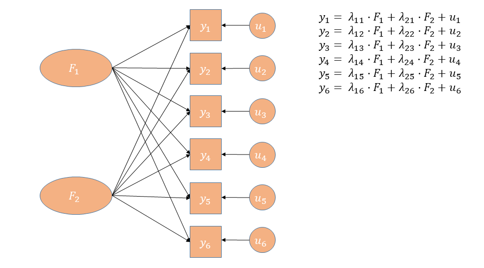
thinking in diagrams (4)
PCA vs EFA

PCA
  • The observed measures are independent variables
    • (arrows go from observed variables to components)
  • The component is a bit like a dependent variable (it’s really just a composite!)
  • Components sequentially capture as much variance in the measures as possible
    • looks for the most variance. doesn’t care if this is variance shared across items, or variance that is unique to a single item.
  • Components are determinate
    • it’s a calculation/transformation. there is one ‘solution’.
EFA
  • The observed measures are dependent variables
    • (arrows go from factors to observed variables)
  • The factor is the independent variable
  • Models the relationships between variables
    • tries to identify shared variance between items, and separate it from variance that is unique to each item.
  • Factors are indeterminate
    • it’s an estimated model, there is no single “correct” solution.

Why prefer EFA over PCA?

  • We give meaning to the new dimensions.

  • Latent factors do not need to be “orthogonal” (uncorrelated)

    • more on this shortly!
  • We learn something.

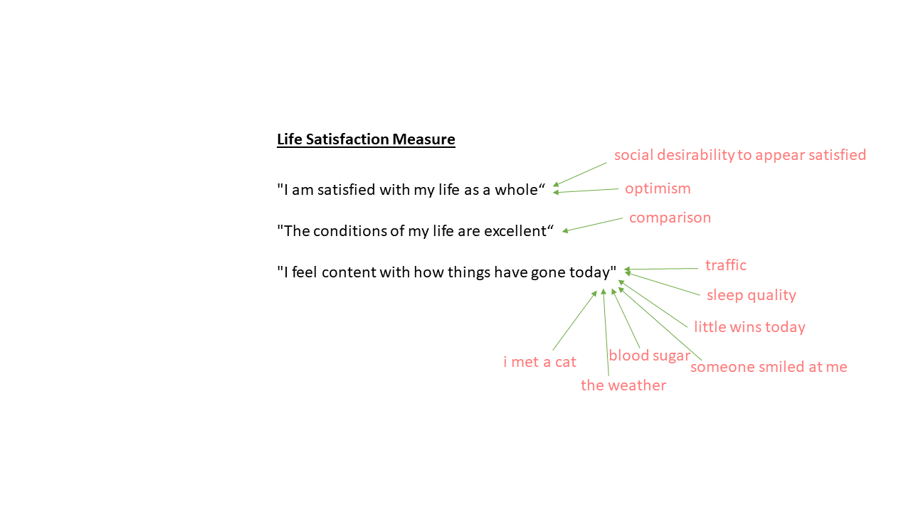
    • are there two different parts to our ‘life satisfaction’ measure, or only 1? or maybe 3?

blurred lines

A little warning..

  • in psychology, people sometimes use PCA and EFA interchangeably!

  • they use PCA but let components correlate, they interpret loadings and give meaning to their components.

  • it’s a rabbit hole that we will not go down..

Activity break

EFA Workflow

Workflow steps

Goal: Reduce, but also learn about/model their underlying (latent) causes

  1. check data
  2. decide “factor extraction method” and “rotation”
  3. how many factors?
  4. define range for nfactors
  5. compare EFAs across the range
  6. if no satisfactory solution, consider removing “problematic” items.
    • If you do, then go back and start over with the reduced set!

How do we fit an EFA in R?

efa

library(psych)
fa(data, nfactors = ?, rotate = ??, fm = ???, cor = ????)

fa()
can take a covariance matrix, a correlation matrix, or the raw data.
nfactors = ?
tells it to estimate a ??? factor model
rotate = ??
tells it whether or not we think those factors could be correlated (more on this shortly)
fm = ???
tells it how to estimate the model
cor = ????
tells it what sort of correlations to use

What does EFA in R look like?

example efa

library(psych)
fa(lsat10[,2:11], nfactors = 4, rotate = "none", fm = "ml", cor = "cor")  
Factor Analysis using method =  ml
Call: fa(r = lsat10[, 2:11], nfactors = 4, rotate = "none", fm = "ml", 
    cor = "cor")
Standardized loadings (pattern matrix) based upon correlation matrix
     ML1   ML2   ML3   ML4   h2    u2 com
Q1  0.53  0.75  0.06  0.05 0.85 0.152 1.8
Q2  0.55  0.70 -0.10 -0.13 0.81 0.187 2.0
Q3  0.96 -0.20 -0.04  0.01 0.96 0.043 1.1
Q4  0.61  0.15  0.11  0.34 0.52 0.483 1.8
Q5  0.87 -0.05 -0.10 -0.09 0.78 0.221 1.1
Q6  0.73 -0.21  0.31 -0.10 0.69 0.310 1.6
Q7  0.19  0.38 -0.23  0.29 0.32 0.681 3.1
Q8  0.53 -0.24  0.25  0.19 0.44 0.563 2.2
Q9  0.25  0.32 -0.09  0.21 0.22 0.779 2.9
Q10 0.38  0.48  0.33 -0.09 0.50 0.505 2.8

                       ML1  ML2  ML3  ML4
SS loadings           3.69 1.69 0.37 0.32
Proportion Var        0.37 0.17 0.04 0.03
Cumulative Var        0.37 0.54 0.58 0.61
Proportion Explained  0.61 0.28 0.06 0.05
Cumulative Proportion 0.61 0.89 0.95 1.00

Mean item complexity =  2
Test of the hypothesis that 4 factors are sufficient.

df null model =  45  with the objective function =  5.22 with Chi Square =  495
df of  the model are 11  and the objective function was  0.09 

The root mean square of the residuals (RMSR) is  0.02 
The df corrected root mean square of the residuals is  0.05 

The harmonic n.obs is  100 with the empirical chi square  2.31  with prob <  1 
The total n.obs was  100  with Likelihood Chi Square =  8.27  with prob <  0.69 

Tucker Lewis Index of factoring reliability =  1.03
RMSEA index =  0  and the 90 % confidence intervals are  0 0.083
BIC =  -42.4
Fit based upon off diagonal values = 1
Measures of factor score adequacy             
                                                   ML1  ML2   ML3   ML4
Correlation of (regression) scores with factors   0.98 0.94  0.69  0.63
Multiple R square of scores with factors          0.97 0.89  0.48  0.40
Minimum correlation of possible factor scores     0.94 0.79 -0.04 -0.20

Example: are you not satisfied?

data

lsat10 <- read_csv("https://uoepsy.github.io/dapr3/2627/misc/lsatdat2.csv")
head(lsat10)
# A tibble: 6 × 11
  id       Q1    Q2    Q3    Q4    Q5    Q6    Q7    Q8    Q9   Q10
  <chr> <dbl> <dbl> <dbl> <dbl> <dbl> <dbl> <dbl> <dbl> <dbl> <dbl>
1 P001     40    50    20    51    15     0    35     1    27    42
2 P002     30    40    70    22    56    62    24    32     2    15
3 P003     77    72    56    71    67    43    63    32    65    75
4 P004     65    60    90    42    64    74    38    34    23    51
5 P005     57    56    39    46    23    33    54     8    35    31
6 P006     41    41    26    26     4    45    12    25    14    67
Data Dictionary
variable description
id Participant ID
Q1 Overall, I am satisfied with my life.
Q2 The conditions of my life are excellent.
Q3 I feel content with how things have gone today.
Q4 I am deeply happy with the way my life has turned out.
Q5 I feel a sense of inner peace and satisfaction.
Q6 I wake up most mornings feeling positive about the day ahead.
Q7 I have gotten the important things I want in life.
Q8 I experience joy and pleasure regularly in my daily life.
Q9 My life has turned out better than I expected it would.
Q10 If I could live my life over, I would change almost nothing.

1/6 Is the data suitable?

  • in short, are items sufficiently correlated with one another?

  • if variables have <5 response options, Pearson’s correlation is not idea. use polychoric correlations instead: fa(......, cor = "poly")

2/6 “factor extraction methods”?

briefly:

  • there are different ways to “extract” (estimate) EFA models.

  • different methods have different requirements, making them more suitable for specific scenarios

  • The default (fm = "minres") is a safe choice

2/6 “rotations”?

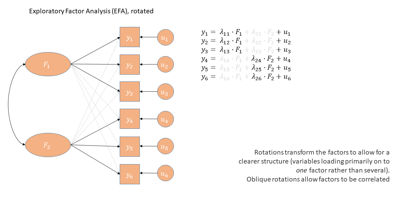
  • Factor rotation is an approach that aims to clarify the relationships between items and factors.

    • Rotation aims to create a ‘simple structure’, where each variable is strongly related to one factor and less to others.
2/6 Why rotate?

  • Without rotation, EFA and PCA are very similar

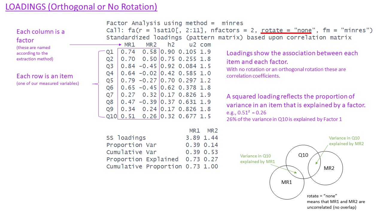
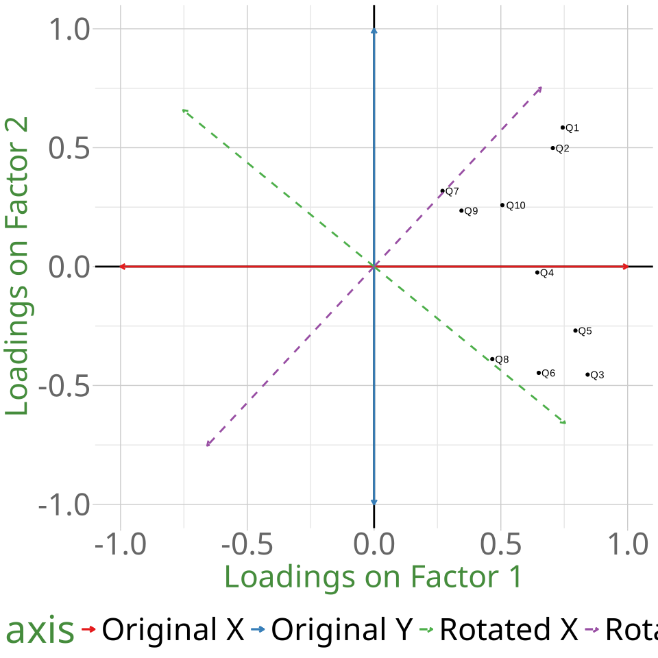
  • Rotation is essentially a transformation applied to the loadings.

  • it doesn’t change the model fit. like scaling a predictor in a lm()
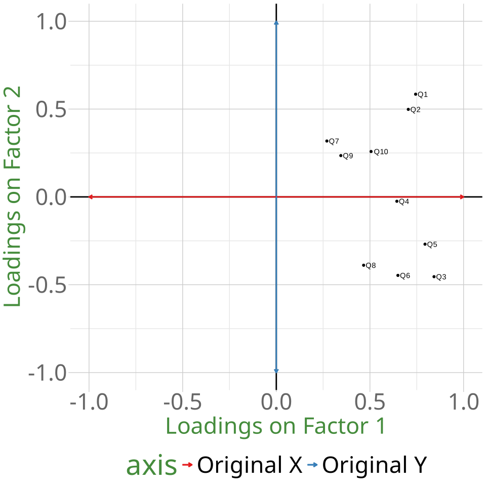
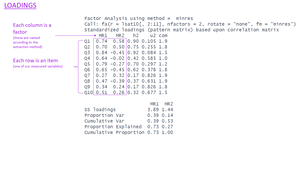
no rotation

fa(lsat10[,2:11], nfactors=2,
   rotate = "none", fm="minres")$loadings |>
   print(cutoff = 0.3)

Loadings:
    MR1    MR2   
Q1   0.744  0.585
Q2   0.705  0.498
Q3   0.842 -0.454
Q4   0.644       
Q5   0.794       
Q6   0.649 -0.447
Q7          0.318
Q8   0.466 -0.389
Q9   0.345       
Q10  0.506       

                 MR1   MR2
SS loadings    3.892 1.444
Proportion Var 0.389 0.144
Cumulative Var 0.389 0.534

2/6 Which rotation?

  • “Orthogonal rotations” keep factors uncorrelated
  • methods include rotate = "varimax" and rotate = "quartimax"
  • Use if you really need factors to be independent (unlikely!)
orthogonal

fa(lsat10[,2:11], nfactors=2,
   rotate = "varimax", fm="minres")$loadings |>
   print(cutoff = 0.3)

Loadings:
    MR1    MR2   
Q1          0.930
Q2          0.839
Q3   0.933       
Q4   0.501  0.405
Q5   0.775  0.320
Q6   0.783       
Q7          0.417
Q8   0.607       
Q9          0.404
Q10         0.528

                 MR1   MR2
SS loadings    2.832 2.504
Proportion Var 0.283 0.250
Cumulative Var 0.283 0.534

2/6 Which rotation?

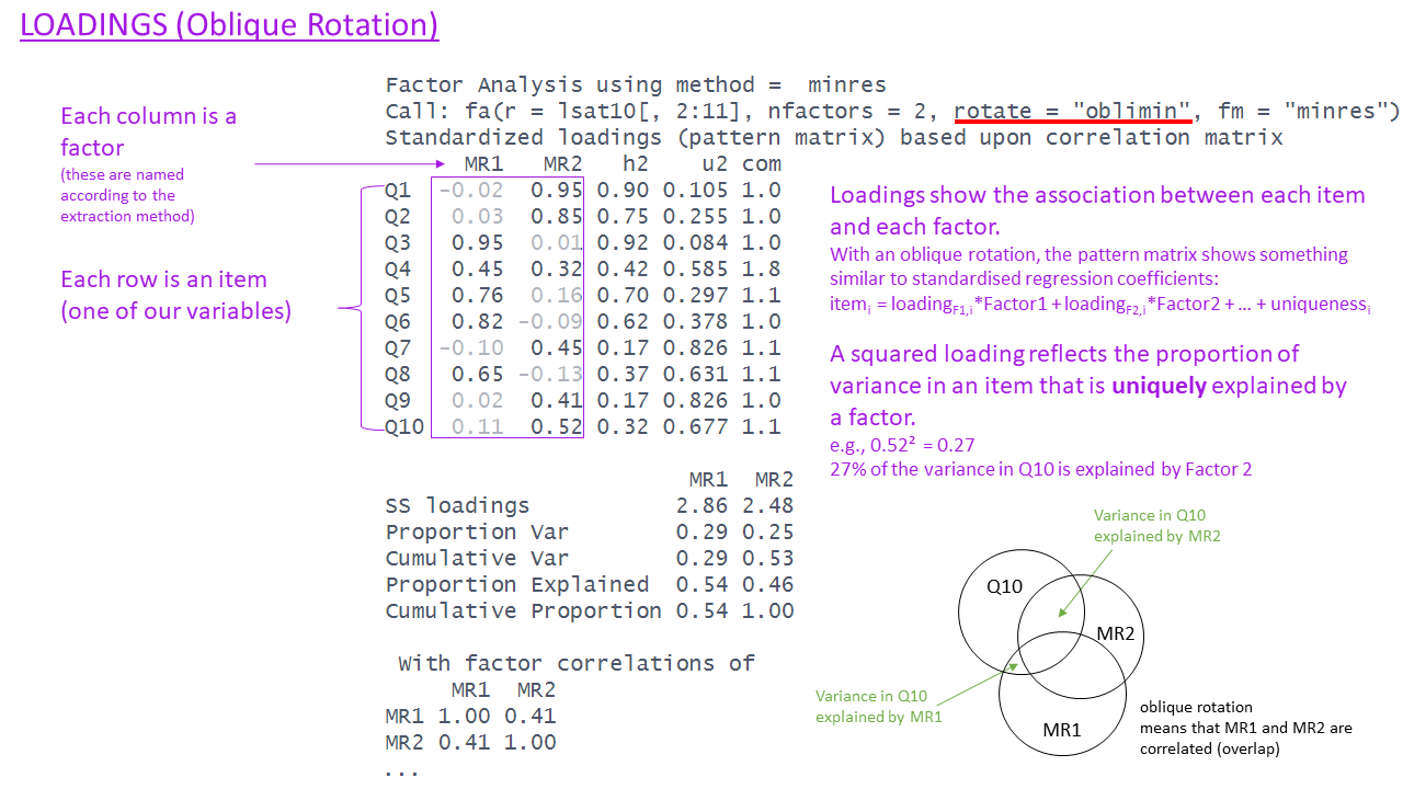
  • “Oblique rotations” allow factors to correlate
  • methods include rotate = "oblimin" and rotate = "promax"
  • Use if you think your factors could be correlated
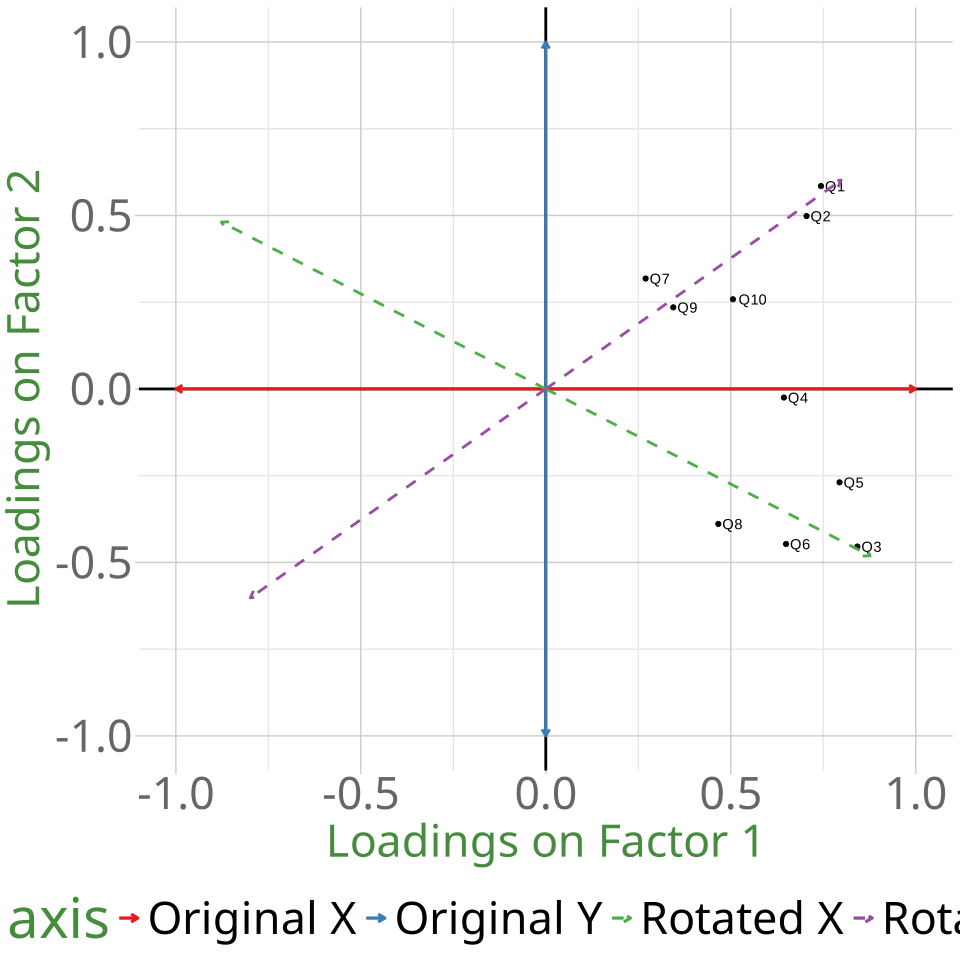
oblique

fa(lsat10[,2:11], nfactors=2,
   rotate = "oblimin", fm="minres")$loadings |>
   print(cutoff = 0.3)

Loadings:
    MR2    MR1   
Q1          0.955
Q2          0.851
Q3   0.954       
Q4   0.447  0.316
Q5   0.760       
Q6   0.820       
Q7          0.448
Q8   0.649       
Q9          0.408
Q10         0.515

                MR2   MR1
SS loadings    2.80 2.418
Proportion Var 0.28 0.242
Cumulative Var 0.28 0.522
 With factor correlations of 
     MR1  MR2
MR1 1.00 0.41
MR2 0.41 1.00

2/6 Which rotation?

  • Do we want to allow our factors to correlate?
    • easy answer: yes. it doesn’t mean they have to..
  • Go with an oblique rotation

3/6 How many factors?

  • Scree plots
  • Parallel Analysis
  • MAP

how many factors?

scree(lsat10[,2:11])

fa.parallel(lsat10[,2:11])

VSS(lsat10[,2:11], plot = FALSE)
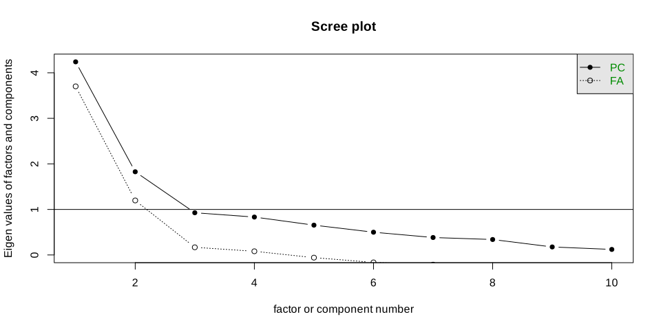
4/6 Determining a range

We want a range, to consider different possible models.

  • Take MAP as a minimum

  • Take Parallel analysis as a maximum

  • if all methods suggest the same number, take 1 either side.

  • We will explore all solutions in this range and select the one that yields the best numerically and theoretically.

5/6 Compare and contrast!

1 factor model

fa(lsat10[,2:11], 
          nfactors = 1, 
          fm = "minres", 
          # rotate = ..
          cor = "cor")
Factor Analysis using method =  minres
Call: fa(r = lsat10[, 2:11], nfactors = 1, fm = "minres", cor = "cor")
Standardized loadings (pattern matrix) based upon correlation matrix
     MR1   h2   u2 com
Q1  0.67 0.46 0.54   1
Q2  0.66 0.44 0.56   1
Q3  0.81 0.66 0.34   1
Q4  0.67 0.44 0.56   1
Q5  0.80 0.65 0.35   1
Q6  0.63 0.40 0.60   1
Q7  0.27 0.07 0.93   1
Q8  0.46 0.22 0.78   1
Q9  0.35 0.12 0.88   1
Q10 0.50 0.25 0.75   1

                MR1
SS loadings    3.70
Proportion Var 0.37

Mean item complexity =  1
Test of the hypothesis that 1 factor is sufficient.

df null model =  45  with the objective function =  5.22 with Chi Square =  495
df of  the model are 35  and the objective function was  2.2 

The root mean square of the residuals (RMSR) is  0.14 
The df corrected root mean square of the residuals is  0.16 

The harmonic n.obs is  100 with the empirical chi square  94.4  with prob <  0.00000023 
The total n.obs was  100  with Likelihood Chi Square =  208  with prob <  2.2e-26 

Tucker Lewis Index of factoring reliability =  0.503
RMSEA index =  0.222  and the 90 % confidence intervals are  0.194 0.253
BIC =  46.3
Fit based upon off diagonal values = 0.86
Measures of factor score adequacy             
                                                   MR1
Correlation of (regression) scores with factors   0.94
Multiple R square of scores with factors          0.88
Minimum correlation of possible factor scores     0.77

2 factor model

fa(lsat10[,2:11], 
          nfactors = 2, 
          fm = "minres", 
          rotate = "oblimin",
          cor = "cor")
Factor Analysis using method =  minres
Call: fa(r = lsat10[, 2:11], nfactors = 2, rotate = "oblimin", fm = "minres", 
    cor = "cor")
Standardized loadings (pattern matrix) based upon correlation matrix
      MR1   MR2   h2    u2 com
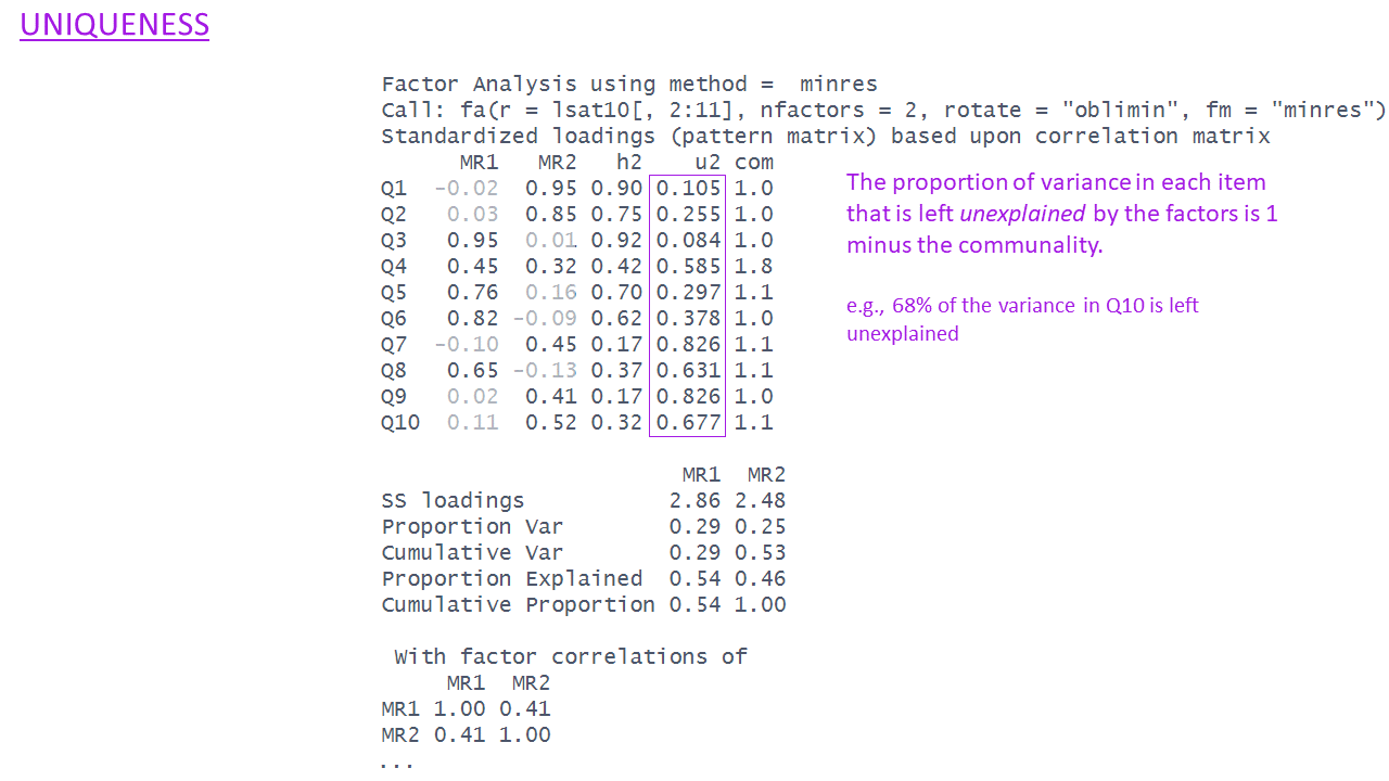
Q1  -0.02  0.95 0.90 0.105 1.0
Q2   0.03  0.85 0.75 0.255 1.0
Q3   0.95  0.01 0.92 0.084 1.0
Q4   0.45  0.32 0.42 0.585 1.8
Q5   0.76  0.16 0.70 0.297 1.1
Q6   0.82 -0.09 0.62 0.378 1.0
Q7  -0.10  0.45 0.17 0.826 1.1
Q8   0.65 -0.13 0.37 0.631 1.1
Q9   0.02  0.41 0.17 0.826 1.0
Q10  0.11  0.52 0.32 0.677 1.1

                       MR1  MR2
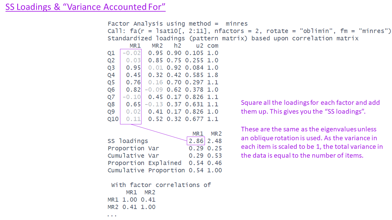
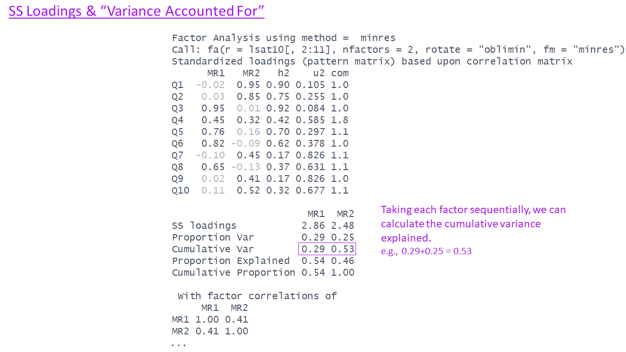
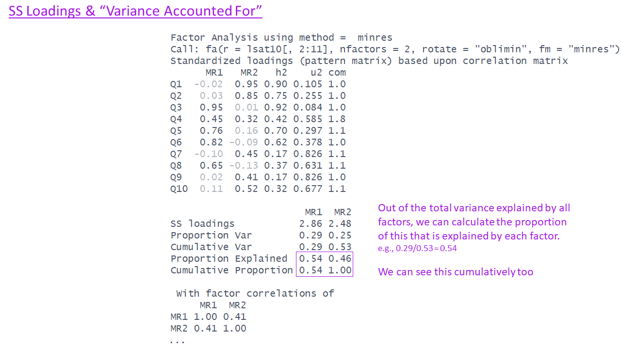
SS loadings           2.86 2.48
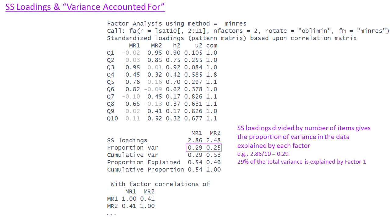
Proportion Var        0.29 0.25
Cumulative Var        0.29 0.53
Proportion Explained  0.54 0.46
Cumulative Proportion 0.54 1.00

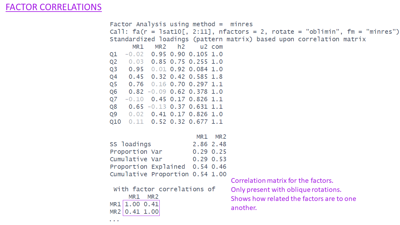
 With factor correlations of 
     MR1  MR2
MR1 1.00 0.41
MR2 0.41 1.00

Mean item complexity =  1.1
Test of the hypothesis that 2 factors are sufficient.

df null model =  45  with the objective function =  5.22 with Chi Square =  495
df of  the model are 26  and the objective function was  0.4 

The root mean square of the residuals (RMSR) is  0.04 
The df corrected root mean square of the residuals is  0.06 

The harmonic n.obs is  100 with the empirical chi square  8.68  with prob <  1 
The total n.obs was  100  with Likelihood Chi Square =  37.8  with prob <  0.063 

Tucker Lewis Index of factoring reliability =  0.954
RMSEA index =  0.067  and the 90 % confidence intervals are  0 0.112
BIC =  -81.9
Fit based upon off diagonal values = 0.99
Measures of factor score adequacy             
                                                   MR1  MR2
Correlation of (regression) scores with factors   0.95 0.95
Multiple R square of scores with factors          0.90 0.90
Minimum correlation of possible factor scores     0.80 0.80

3 factor model

fa(lsat10[,2:11], 
          nfactors = 3, 
          fm = "minres", 
          rotate = "oblimin",
          cor = "cor")
Factor Analysis using method =  minres
Call: fa(r = lsat10[, 2:11], nfactors = 3, rotate = "oblimin", fm = "minres", 
    cor = "cor")
Standardized loadings (pattern matrix) based upon correlation matrix
      MR2   MR1   MR3   h2    u2 com
Q1  -0.02  0.95  0.02 0.90 0.104 1.0
Q2   0.05  0.82  0.07 0.73 0.270 1.0
Q3   0.98 -0.03  0.09 0.94 0.065 1.0
Q4   0.49  0.26  0.17 0.44 0.560 1.8
Q5   0.77  0.14  0.06 0.70 0.299 1.1
Q6   0.78  0.00 -0.29 0.72 0.280 1.3
Q7  -0.03  0.35  0.32 0.25 0.746 2.0
Q8   0.63 -0.11 -0.03 0.36 0.639 1.1
Q9   0.09  0.32  0.26 0.22 0.776 2.1
Q10  0.02  0.65 -0.28 0.46 0.536 1.4

                       MR2  MR1  MR3
SS loadings           2.90 2.43 0.40
Proportion Var        0.29 0.24 0.04
Cumulative Var        0.29 0.53 0.57
Proportion Explained  0.51 0.42 0.07
Cumulative Proportion 0.51 0.93 1.00

 With factor correlations of 
      MR2  MR1   MR3
MR2  1.00 0.41 -0.07
MR1  0.41 1.00  0.15
MR3 -0.07 0.15  1.00

Mean item complexity =  1.4
Test of the hypothesis that 3 factors are sufficient.

df null model =  45  with the objective function =  5.22 with Chi Square =  495
df of  the model are 18  and the objective function was  0.26 

The root mean square of the residuals (RMSR) is  0.03 
The df corrected root mean square of the residuals is  0.05 

The harmonic n.obs is  100 with the empirical chi square  4.59  with prob <  1 
The total n.obs was  100  with Likelihood Chi Square =  24.3  with prob <  0.15 

Tucker Lewis Index of factoring reliability =  0.964
RMSEA index =  0.058  and the 90 % confidence intervals are  0 0.114
BIC =  -58.6
Fit based upon off diagonal values = 0.99
Measures of factor score adequacy             
                                                   MR2  MR1   MR3
Correlation of (regression) scores with factors   0.97 0.94  0.67
Multiple R square of scores with factors          0.95 0.88  0.45
Minimum correlation of possible factor scores     0.89 0.75 -0.11

Evaluating factor solutions

Evaluating factor solutions

Variance explained

Identification of factors

Salience of items

Cross-loadings

Heywood cases

Theoretical coherence

… and when in doubt, parsimony

Evaluating factor solutions

>> Variance explained

Identification of factors

Salience of items

Cross-loadings

Heywood cases

Theoretical coherence

… and when in doubt, parsimony

  • how much variance is explained by the solution?
  • how much by each of the factors?

Evaluating factor solutions

Variance explained

>> Identification of factors

Salience of items

Cross-loadings

Heywood cases

Theoretical coherence

… and when in doubt, parsimony

V

  • does each factor have \(\ge 3\) items with it as their primary loading?
  • factors with \(< 3\) items suggests you may have too many factors!

Evaluating factor solutions

Variance explained

Identification of factors

>> Salience of items

Cross-loadings

Heywood cases

Theoretical coherence

… and when in doubt, parsimony

V

I

  • do all items have at least one loading at a salient level?
  • in most research “salient” is \(\ge|.3|\) or \(\ge|.4|\)
  • items with no salient loadings may indicate:
    • a problem item
    • too few factors

Evaluating factor solutions

Variance explained

Identification of factors

Salience of items

>> Cross-loadings

Heywood cases

Theoretical coherence

… and when in doubt, parsimony

V

I

S

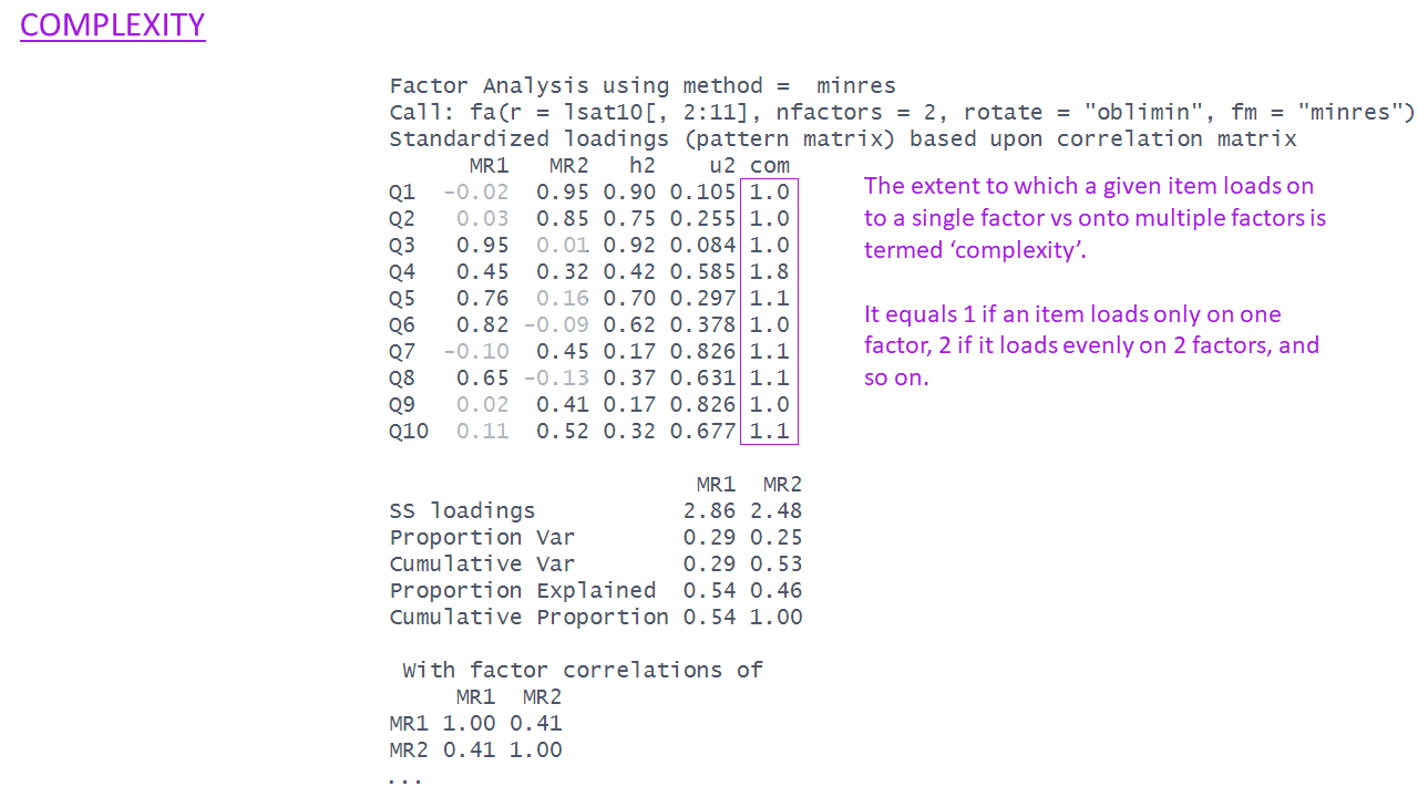
  • are there any items with multiple salient loadings?
  • these are “complex” items (see the complexity column)
  • they make it harder to define the factors
  • cross-loadings may indicate:
    • a problem item
    • too few factors

Evaluating factor solutions

Variance explained

Identification of factors

Salience of items

Cross-loadings

>> Heywood cases

Theoretical coherence

… and when in doubt, parsimony

V

I

S

C

  • “Heywood cases” are communalities or factor loadings that are >1 (i.e., impossible values.
  • these are definitely a problem!
  • consider:
    • a different extraction method
    • eliminating items
    • rethinking if EFA is what you actually want

Evaluating factor solutions

Variance explained

Identification of factors

Salience of items

Cross-loadings

Heywood cases

>> Theoretical coherence

… and when in doubt, parsimony

V

I

S

C

H

  • is the factor structure (items that load on to each factor) coherent, and does it make theoretical sense?
  • can you give a name to each factor?

5/6 Compare and contrast!

1 factor model TEST

fa1 <- fa(lsat10[,2:11], 
          nfactors = 1, 
          fm = "minres", 
          # rotate = ..
          cor = "cor")
          
print(fa1$loadings,
        cutoff = 0.3,
        sort = TRUE)

Loadings:
    MR1  
Q1  0.675
Q2  0.661
Q3  0.812
Q4  0.666
Q5  0.804
Q6  0.632
Q10 0.505
Q7       
Q8  0.464
Q9  0.347

                MR1
SS loadings    3.70
Proportion Var 0.37

2 factor model

fa2 <- fa(lsat10[,2:11], 
          nfactors = 2, 
          fm = "minres", 
          rotate = "oblimin",
          cor = "cor")

print(fa2$loadings,
        cutoff = 0.3,
        sort = TRUE)

Loadings:
    MR2    MR1   
Q3   0.954       
Q5   0.760       
Q6   0.820       
Q8   0.649       
Q1          0.955
Q2          0.851
Q10         0.515
Q4   0.447  0.316
Q7          0.448
Q9          0.408

                MR2   MR1
SS loadings    2.80 2.418
Proportion Var 0.28 0.242
Cumulative Var 0.28 0.522

3 factor model

fa3 <- fa(lsat10[,2:11], 
          nfactors = 3, 
          fm = "minres", 
          rotate = "oblimin",
          cor = "cor")

print(fa3$loadings,
        cutoff = 0.3,
        sort = TRUE)

Loadings:
    MR1    MR2    MR3   
Q3   0.982              
Q5   0.772              
Q6   0.777              
Q8   0.634              
Q1          0.950       
Q2          0.820       
Q10         0.655       
Q4   0.492              
Q7          0.349  0.322
Q9          0.320       

                 MR1   MR2   MR3
SS loadings    2.818 2.326 0.380
Proportion Var 0.282 0.233 0.038
Cumulative Var 0.282 0.514 0.552

5/6 Compare and contrast!

1 factor model

fa1 <- fa(lsat10[,2:11], 
          nfactors = 1, 
          fm = "minres", 
          # rotate = ..
          cor = "cor")
          
print(fa1$loadings,
        cutoff = 0.3,
        sort = TRUE)

Loadings:
    MR1  
Q1  0.675
Q2  0.661
Q3  0.812
Q4  0.666
Q5  0.804
Q6  0.632
Q10 0.505
Q7       
Q8  0.464
Q9  0.347

                MR1
SS loadings    3.70
Proportion Var 0.37

2 factor model

fa2 <- fa(lsat10[,2:11], 
          nfactors = 2, 
          fm = "minres", 
          rotate = "oblimin",
          cor = "cor")

print(fa2$loadings,
        cutoff = 0.3,
        sort = TRUE)

Loadings:
    MR1    MR2   
Q3   0.954       
Q5   0.760       
Q6   0.820       
Q8   0.649       
Q1          0.955
Q2          0.851
Q10         0.515
Q4   0.447  0.316
Q7          0.448
Q9          0.408

                MR1   MR2
SS loadings    2.80 2.418
Proportion Var 0.28 0.242
Cumulative Var 0.28 0.522
Data Dictionary
variable description
id Participant ID
Q1 Overall, I am satisfied with my life.
Q2 The conditions of my life are excellent.
Q3 I feel content with how things have gone today.
Q4 I am deeply happy with the way my life has turned out.
Q5 I feel a sense of inner peace and satisfaction.
Q6 I wake up most mornings feeling positive about the day ahead.
Q7 I have gotten the important things I want in life.
Q8 I experience joy and pleasure regularly in my daily life.
Q9 My life has turned out better than I expected it would.
Q10 If I could live my life over, I would change almost nothing.

6/6 Removal of items?

identification

some items could turn out to be:

  • irrelevant
    • low factor loadings/communalities that add noise without contributing to a factor
  • more complex/ambiguous
    • crossloadings that obscure clear interpretation

watch out - both of these could also mean we don’t have enough factors!

what to do

  1. EXAMINE THE ITEMS!
  • check for double barreled phrasing, vague language etc.
  1. iterative removal (one by one), re-doing steps 1-5 each time.

Cautions!

💩 The “garbage in garbage out” principle always applies

  • PCA and factor analysis cannot turn bad data into good data

  • If one or more factors don’t make sense, then either the items are bad, the theory is bad, the analysis is bad, or all three are bad!

Extras

Example factor models

The –insert name here– scale

I went through the responses from last week, and pulled out these recurring themes:

  • ethical & societal concerns (environmental, corporate)
  • accuracy / reliability (or lack thereof!)
  • efficiency
  • ease of use
  • (lack of) humanity
  • social pressure

What we need now:

  • questions!
  • a name!


https://edin.ac/4jVggSE