Interpreting LMMs and
building maximal models

Data Analysis for Psychology in R 3

Elizabeth Pankratz (elizabeth.pankratz@ed.ac.uk)

Department of Psychology
University of Edinburgh
2026–2027

Course Overview

Linear mixed models (with Dr. Elizabeth Pankratz)	Regression refresher, intro to group-structured data
	Modelling group-structured data using random effects
	Interpreting LMMs and building maximal models
	Troubleshooting model fit, checking assumptions + diagnostics
	LMMs: Practice analysis
factor analysis working with multi-item measures (with Dr. Josiah King)	measurement and dimensionality
	exploring underlying constructs (EFA)
	testing theoretical models (CFA)
	reliability and validity
	recap & exam prep

Reminder: Fill in the skill-ranking form so we can create report groups

Please fill in the form by noon (12 pm) on Wednesday, 7 October!

https://edin.ac/4rOgRHB

You’ll find out about your group allocation on Thursday, 8 October.

You already can see the general report instructions and rubric on Learn under Assessment > Report >
Report Overview & FAQ.

The analysis task itself will be released at noon on Thursday 8 October.

For lots of guidance, check the flashcards:

• LMM analysis workflow (you’ll see many of these steps today!)
• Report LMM analyses and results

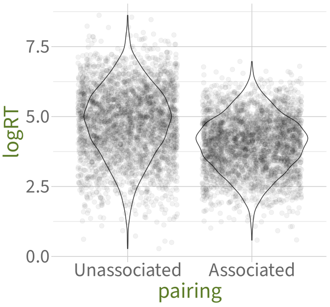
Same data as before: Log reaction times in the
Implicit Association Test (IAT)

set.seed(1)
implicit_data |>
  ggplot(aes(x = pairing, y = logRT)) +
  geom_violin() +
  geom_jitter(alpha = 0.05, size = 3) +
  NULL

implicit_data |>
  head(12)

# A tibble: 12 x 4
   ppt_id item_id pairing      logRT
   <chr>  <chr>   <fct>        <dbl>
 1 ppt1   item1   Associated    4.33
 2 ppt1   item1   Unassociated  4.70
 3 ppt2   item1   Associated    4.17
 4 ppt2   item1   Unassociated  4.91
 5 ppt3   item1   Associated    4.45
 6 ppt3   item1   Unassociated  5.13
 7 ppt4   item1   Associated    4.41
 8 ppt4   item1   Unassociated  6.54
 9 ppt5   item1   Associated    5.19
10 ppt5   item1   Unassociated  6.64
11 ppt6   item1   Associated    4.74
12 ppt6   item1   Unassociated  5.96

Why is a simple linear model not appropriate for this data?

This week’s learning objectives

How do we interpret the random effects part of a model summary?

How do we know if a model can include random intercepts for a given grouping variable?

How do we know if a model can include random slopes over a given predictor for a given grouping variable?

What is a maximal model?

Recap: Linear mixed models (LMMs)

Modelling the IAT data with an LMM

library(lme4)

implicit_full_lmm <- lmer(      # LMMs use lme4::lmer(), not lm()
  
  logRT ~ pairing +             # fixed effects: predict logRT by pairing
                                # (0 = Unassociated, 1 = Associated)
    
                                # random effects:
    (1 + pairing | ppt_id) +    # for each ppt, adjust the intercept and the slope
    
    (1 + pairing | item_id),    # for each item, adjust the intercept and the slope
  
  data = implicit_data
)

What does it mean to “adjust the intercept”?

The average association between logRT and pairing (the line defined by the fixed intercept and fixed slope):

If a participant or an item has a higher log RT than average, then they will have a positive adjustment to the fixed intercept.

If a participant or an item has a lower log RT than average, then they will have a negative adjustment to the fixed intercept.

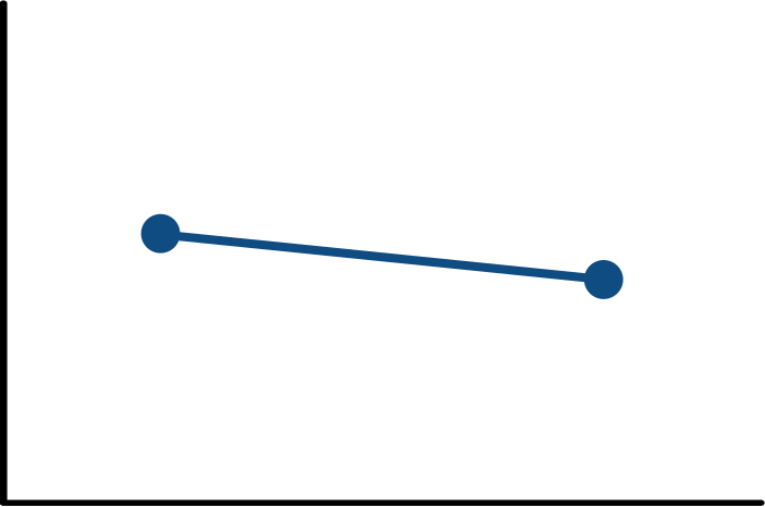
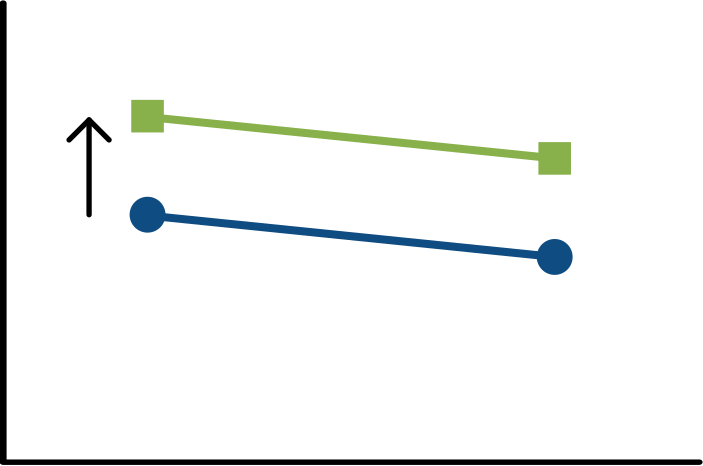
When the model includes random intercepts by ppt_id and by item_id, it will estimate how much the fixed intercept should be nudged up or down, in order to better fit the data from each participant and each item.

What does it mean to “adjust the slope”?

The average association between logRT and pairing (the line defined by the fixed intercept and fixed slope):

If a participant or an item has a more positive effect of pairing than average, then they will have a positive adjustment to the fixed slope over pairing.

If a participant or an item has a more negative effect of pairing than average, then they will have a negative adjustment to the fixed slope over pairing.

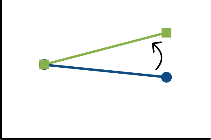
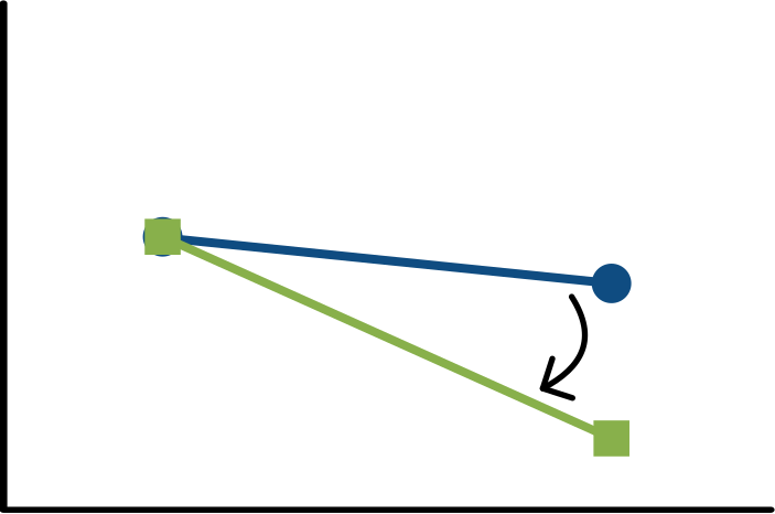
When the model includes random intercepts by ppt_id and by item_id as well as random slopes over pairing by ppt_id and by item_id, it will

• estimate how much the fixed intercept should be nudged up or down (last slide) AND ALSO
• how much the fixed slope should be swung up or down (this slide)

in order to better fit the data from each participant and each item.

Interpreting LMM summaries

The full summary

summary(implicit_full_lmm)

Linear mixed model fit by REML ['lmerMod']
Formula: logRT ~ pairing + (1 + pairing | ppt_id) + (1 + pairing | item_id)
   Data: implicit_data

REML criterion at convergence: 10722

Scaled residuals: 
   Min     1Q Median     3Q    Max 
-3.765 -0.669 -0.005  0.666  3.401 

Random effects:
 Groups   Name              Variance Std.Dev. Corr 
 ppt_id   (Intercept)       0.6068   0.779         
          pairingAssociated 0.0986   0.314    -0.83
 item_id  (Intercept)       0.7759   0.881         
          pairingAssociated 0.1508   0.388    -0.77
 Residual                   0.2730   0.522         
Number of obs: 6400, groups:  ppt_id, 100; item_id, 32

Fixed effects:
                  Estimate Std. Error t value
(Intercept)         4.7713     0.1744   27.37
pairingAssociated  -0.7624     0.0766   -9.95

Correlation of Fixed Effects:
            (Intr)
parngAssctd -0.776

Start with the fixed effects

Fixed effects:
                   Estimate Std. Error t value
 (Intercept)         4.7713     0.1744   27.37
 pairingAssociated  -0.7624     0.0766   -9.95

Interpret the fixed effects the same way you interpret coefficients in a simple linear model.

(Intercept) = the estimated mean outcome when all predictors are equal to zero.

• The estimated mean log reaction time when the topic pairing is unassociated (the reference level, coded as 0) is 4.77 log units.

pairingAssociated = the estimated increase/decrease in the outcome when the predictor moves from 0 to 1.

• The log reaction time for associated pairings is estimated to be 0.76 log units smaller than the log reaction time for unassociated pairings.

Where are the p-values?

Where are the p-values?

The mathematics that make the random effects work (which you do not need to know!) means that we can’t easily translate t-values to p-values. But clever people have come up with good approximations!

Add the approximated p-values into the model summary by

• loading the library lmerTest, and
• re-fitting the LMM using lmer().

This gives you p-values estimated using “Satterthwaite’s method”.

library(lmerTest)

implicit_full_lmm <- lmer(
  logRT ~ pairing +  (1 + pairing | ppt_id) +  (1 + pairing | item_id), 
  data = implicit_data
)

summary(implicit_full_lmm)

...

 Fixed effects:
                   Estimate Std. Error      df t value Pr(>|t|)    
 (Intercept)         4.7713     0.1744 47.4387   27.37  < 2e-16 ***
 pairingAssociated  -0.7624     0.0766 44.0019   -9.95  7.8e-13 ***

...

Fixed effects, now with p-values

 Fixed effects:
                   Estimate Std. Error      df t value Pr(>|t|)    
 (Intercept)         4.7713     0.1744 47.4387   27.37  < 2e-16 ***
 pairingAssociated  -0.7624     0.0766 44.0019   -9.95  7.8e-13 ***

(Intercept):

• The estimated mean log reaction time when the topic pairing is unassociated (the reference level, coded as 0) is 4.77 log units.
• This estimate is significantly different from zero at \(p\) < .001, but that’s not really a surprise … we were already pretty sure that the average log RT would be different from zero!
  • When the outcome variable is continuous, we typically don’t report p-values for intercepts, because it’s not a very interesting hypothesis test

pairingAssociated:

• The log reaction time for associated pairings is estimated to be 0.76 log units smaller than the log reaction time for unassociated pairings.
• This estimate is significantly different from zero (\(p\) < .001).
  • This is an interesting hypothesis test, because it looks at the difference between conditions, which is the whole point of our experiment

Next, look at the random effects

Random effects:
  Groups   Name              Variance Std.Dev. Corr 
  ppt_id   (Intercept)       0.6068   0.779         
           pairingAssociated 0.0986   0.314    -0.83
  item_id  (Intercept)       0.7759   0.881         
           pairingAssociated 0.1508   0.388    -0.77
  Residual                   0.2730   0.522         
 Number of obs: 6400, groups:  ppt_id, 100; item_id, 32
 

First: Sense check the quantities in the final line.

• Is the number of observations (6400) correct?
• Is the number of distinct levels of ppt_id (100) correct?
• Is the number of distinct levels of item_id (32) correct?

If not, the data is probably not formatted correctly. Do any fixes you need.

Then: Look at the rest of the output. Read it row by row as a table, like this:

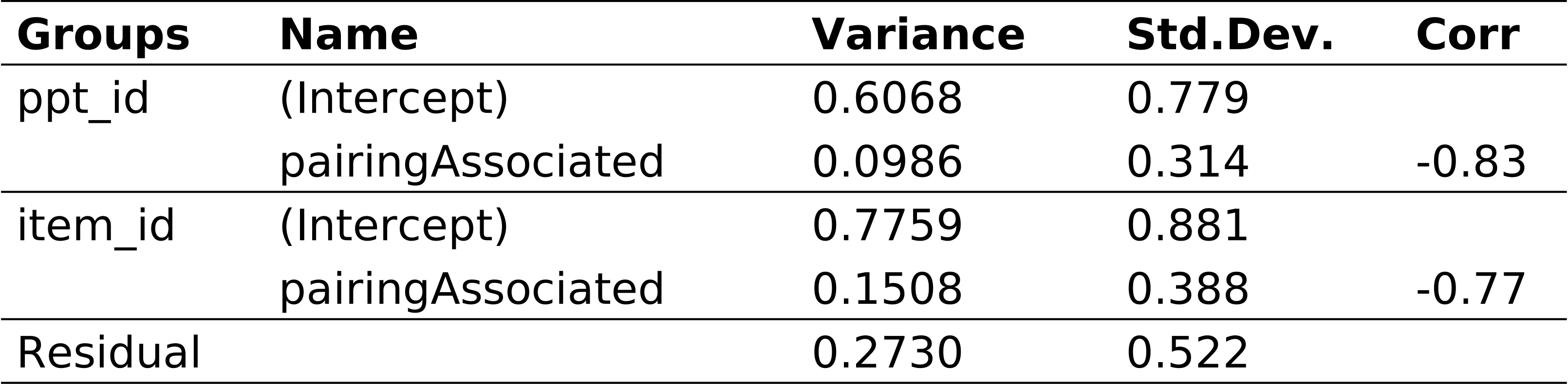
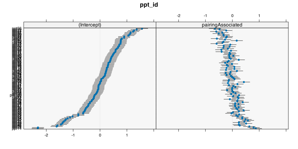
Intercept adjustments for each ppt_id (1)

  Groups   Name              Variance Std.Dev. Corr 
  ppt_id   (Intercept)       0.6068   0.779         

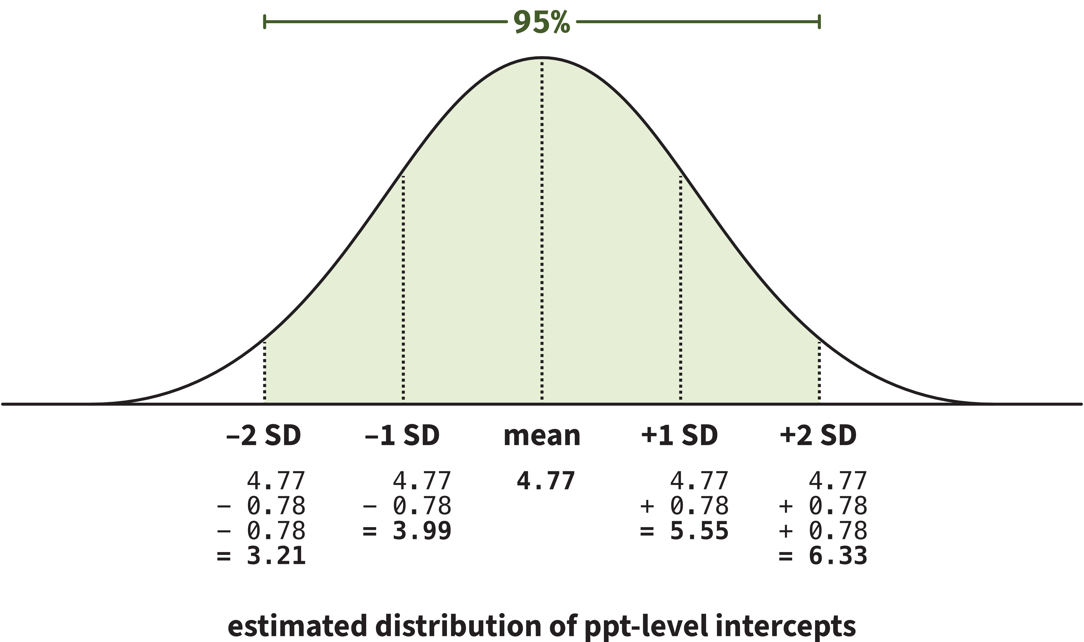
What this line tells us: The (Intercept) adjustments for ppt_id have a standard deviation (SD) of 0.78 log units.

• The variance is just the SD squared (0.779\(^2\) = 0.607) so it doesn’t add any useful information.
• We will always just focus on the SD.

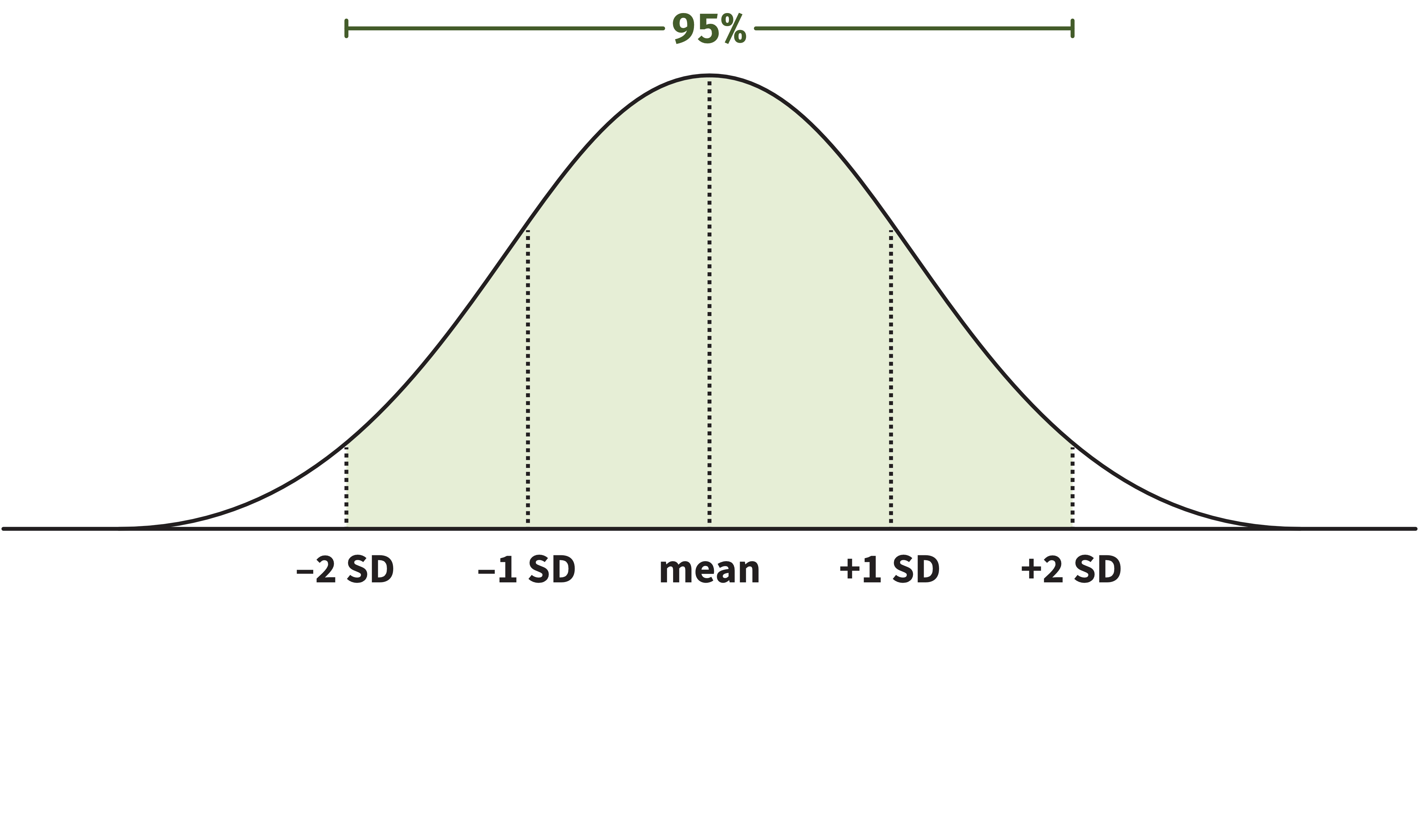
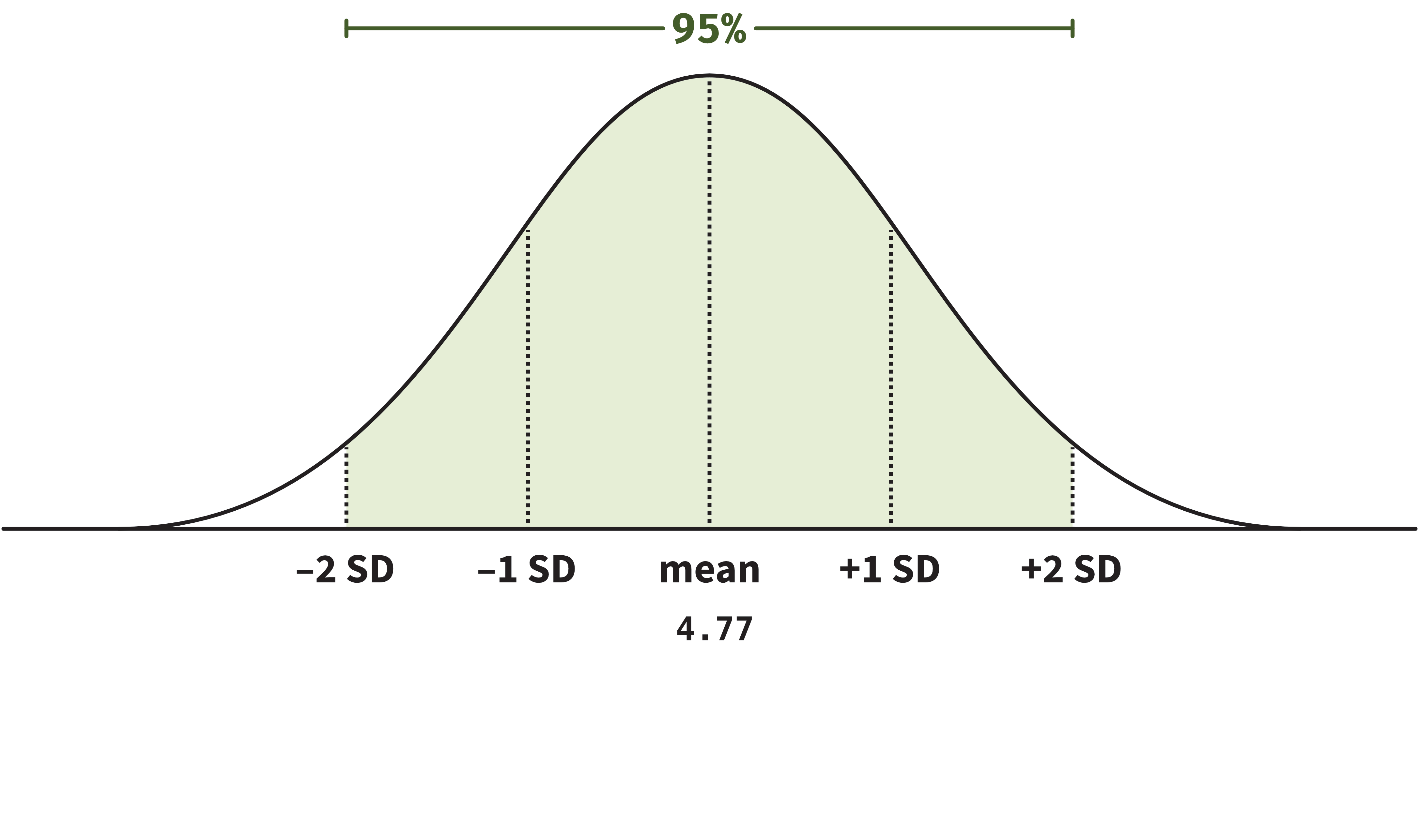
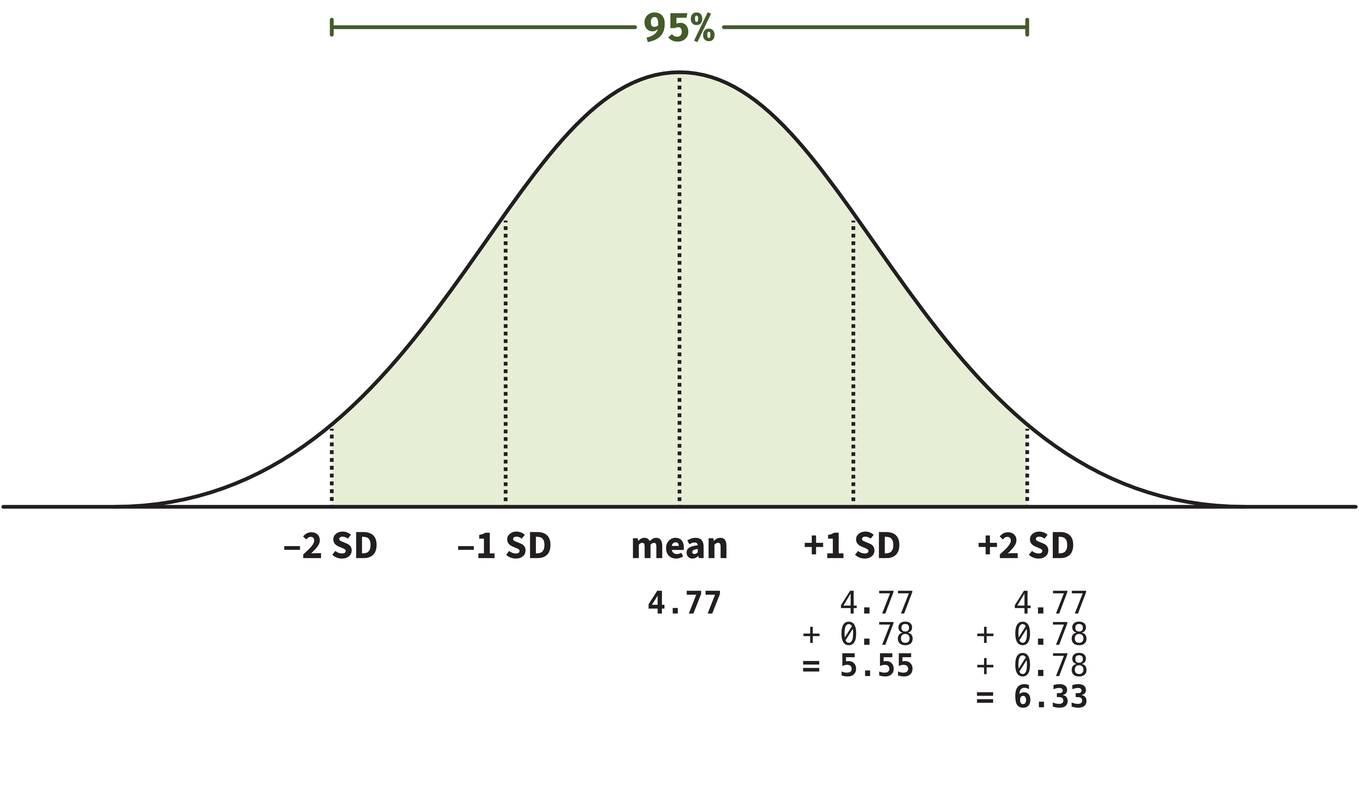
The number 0.78 doesn’t mean much on its own. We must interpret it with respect to the value that it is adjusting: the fixed intercept of 4.77 log units.

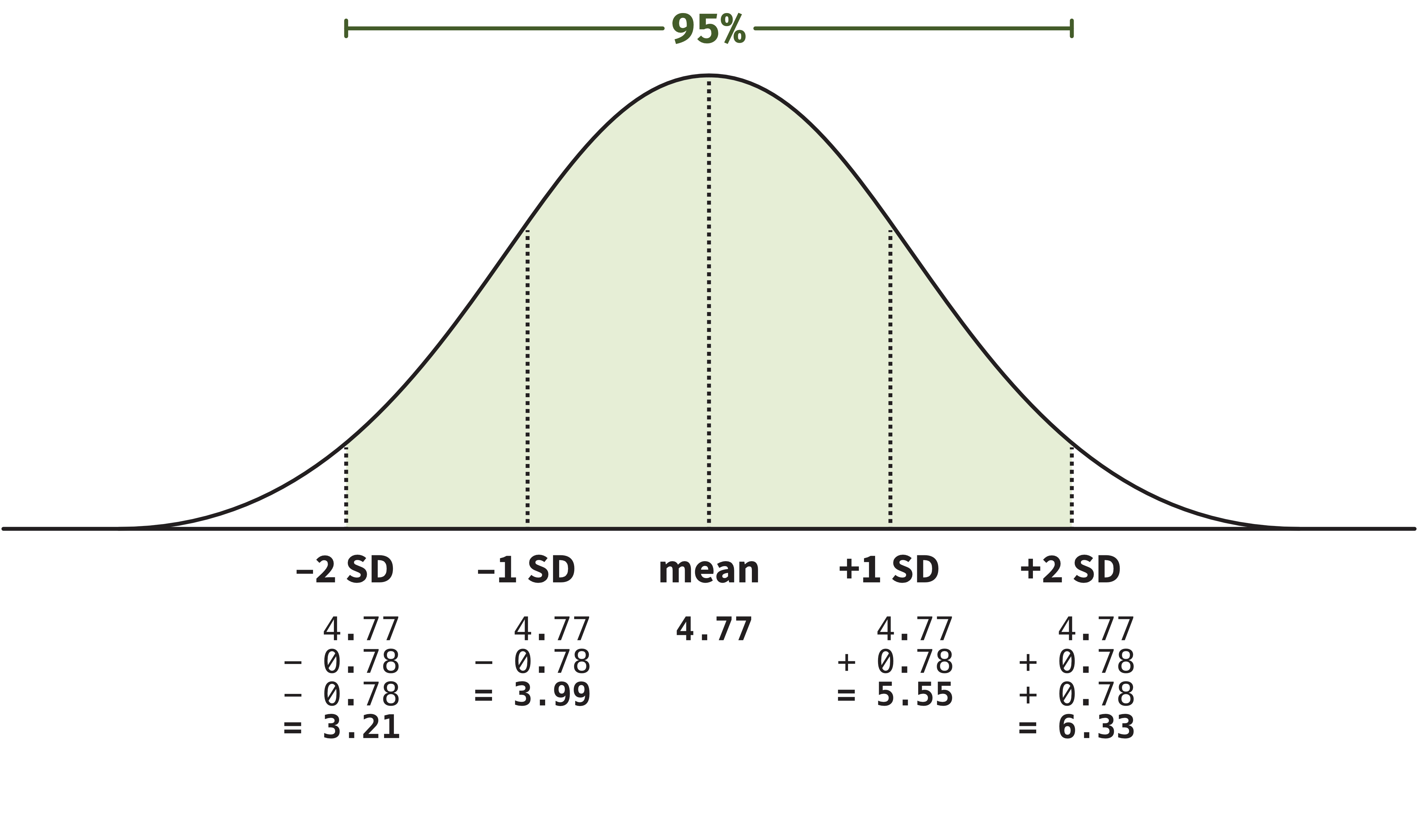
By combining these numbers, we find the estimated distribution of participant-level intercepts.

This is useful because it helps us understand the variability in participant behaviour in our experiment.

Intercept adjustments for each ppt_id (2)

  Groups   Name              Variance Std.Dev. Corr 
  ppt_id   (Intercept)       0.6068   0.779         

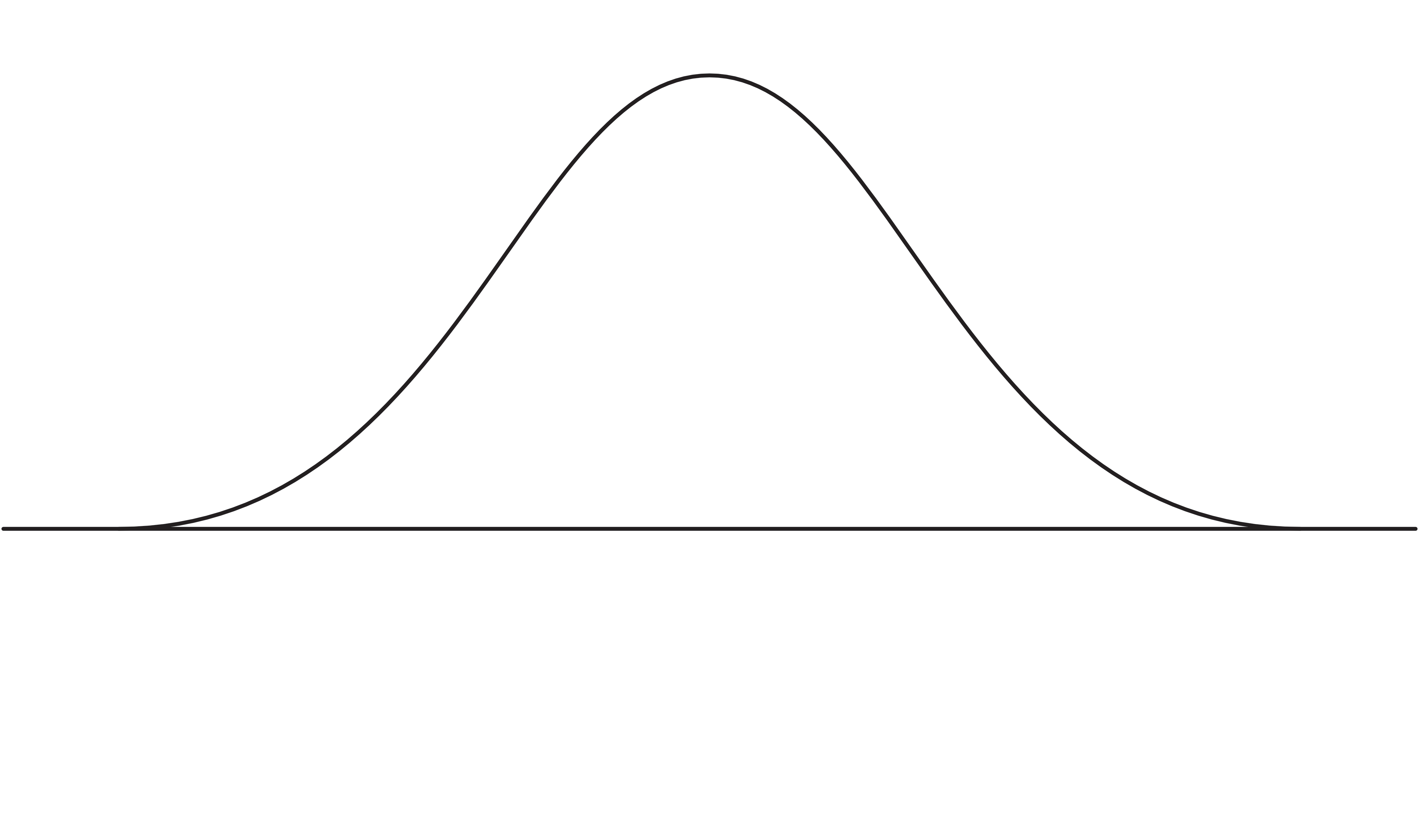
Intercept adjustments for each ppt_id (3)

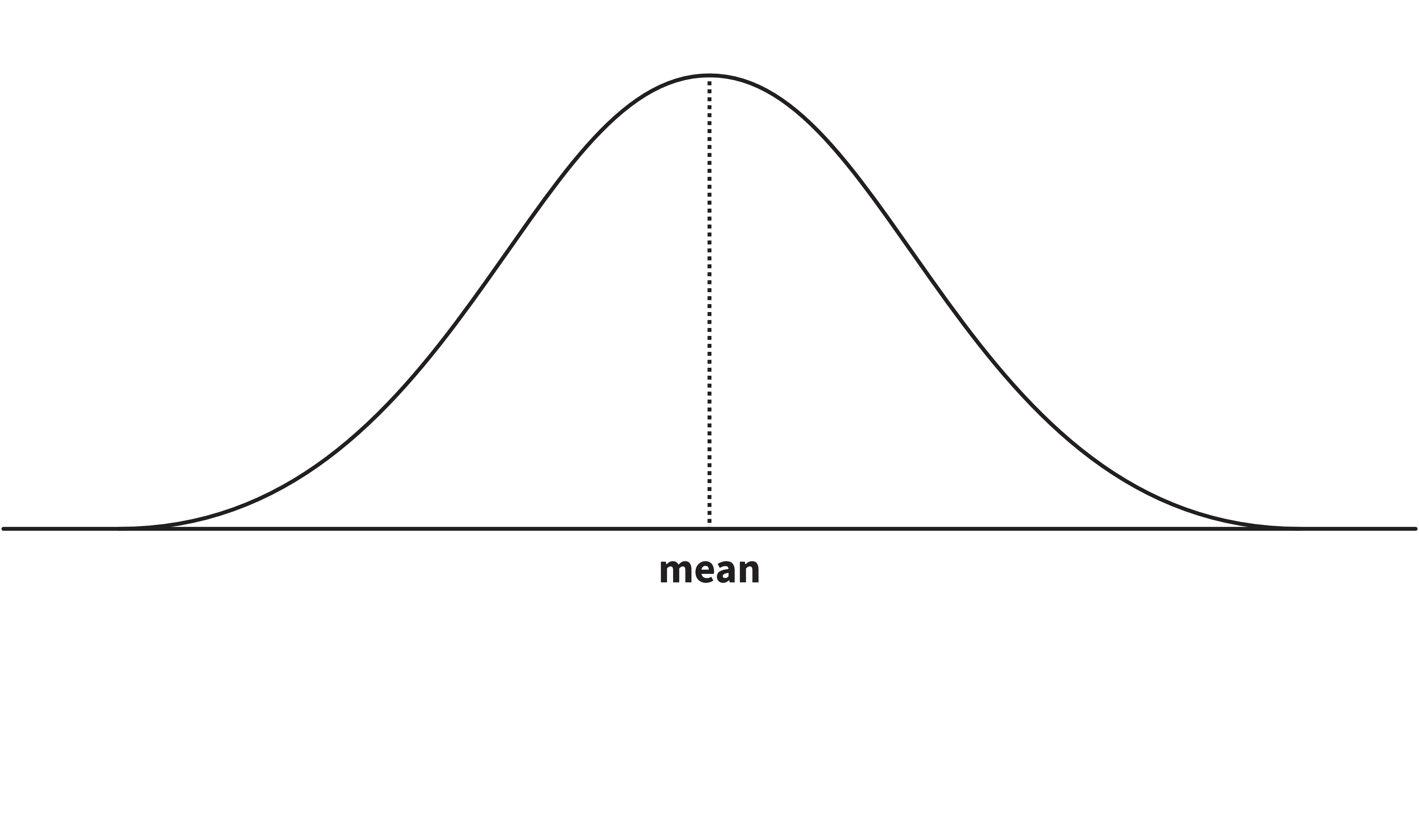
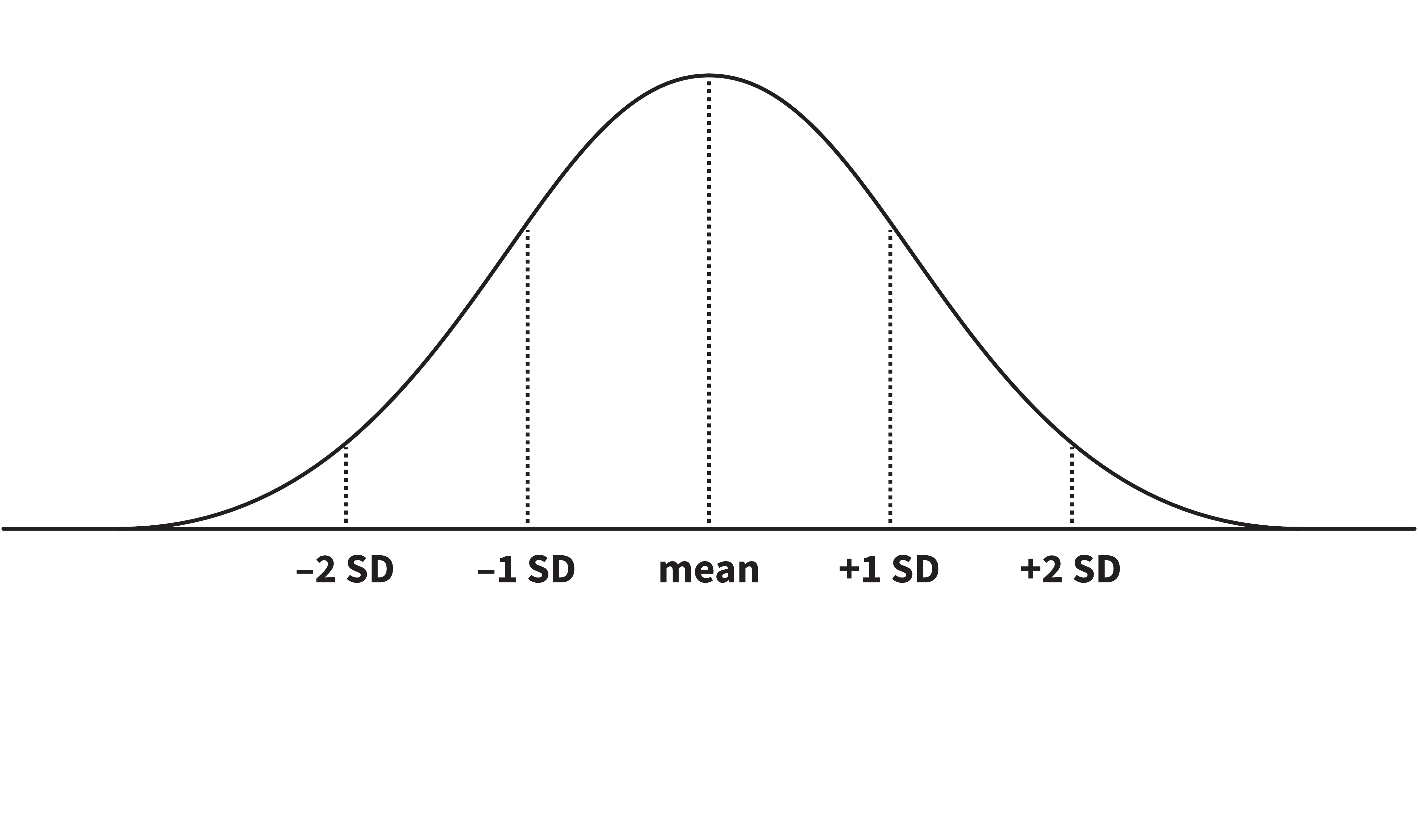
Approx 95% of participant-level intercepts are estimated to fall between about 3.21 log units and 6.33 log units.

This means that, for 95% of participants, the estimated log RT for unassociated pairings is between 3.21 log units and 6.33 log units.

Useful information to report!

pairingAssociated adjustments by ppt_id

  Groups   Name              Variance Std.Dev. Corr 
  ppt_id   (Intercept)       0.6068   0.779         
           pairingAssociated 0.0986   0.314    -0.83

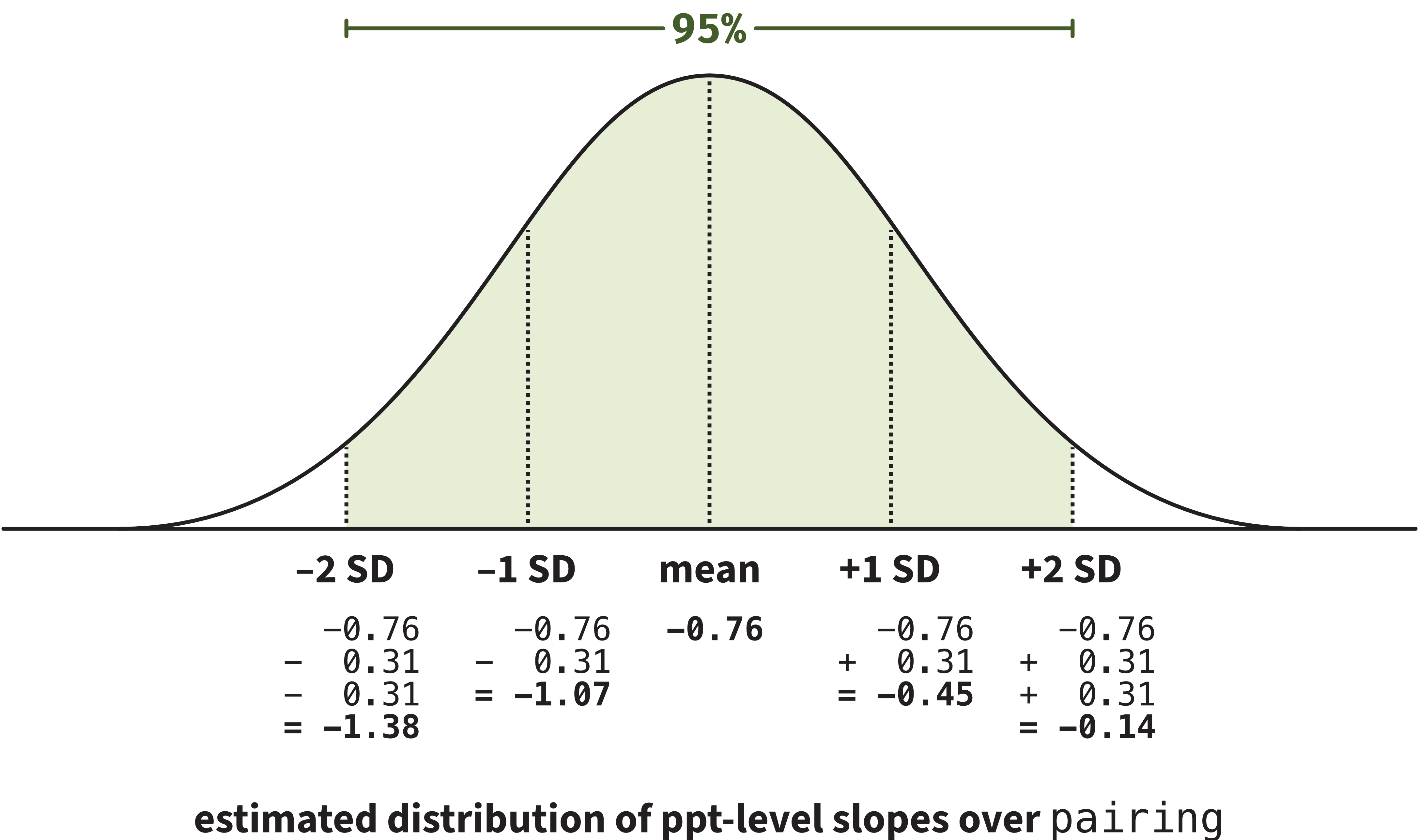
The pairingAssociated adjustments (i.e., adjustments to the slope over pairing) for ppt_id have a SD of 0.31 log units.

At least 95% of participants are estimated to have a negative effect of pairing: faster RTs for associated pairings compared to unassociated pairings.

Correlation between by-participant slope and intercept adjustments

  Groups   Name              Variance Std.Dev. Corr 
  ppt_id   (Intercept)       0.6068   0.779         
           pairingAssociated 0.0986   0.314    -0.83

The participant-level (Intercept) and pairingAssociated adjustments have a correlation of –0.83.

dotplot.ranef.mer(ranef(implicit_full_lmm))$ppt_id

What questions do you have right now?

Over to you for interpreting item_id adjustments

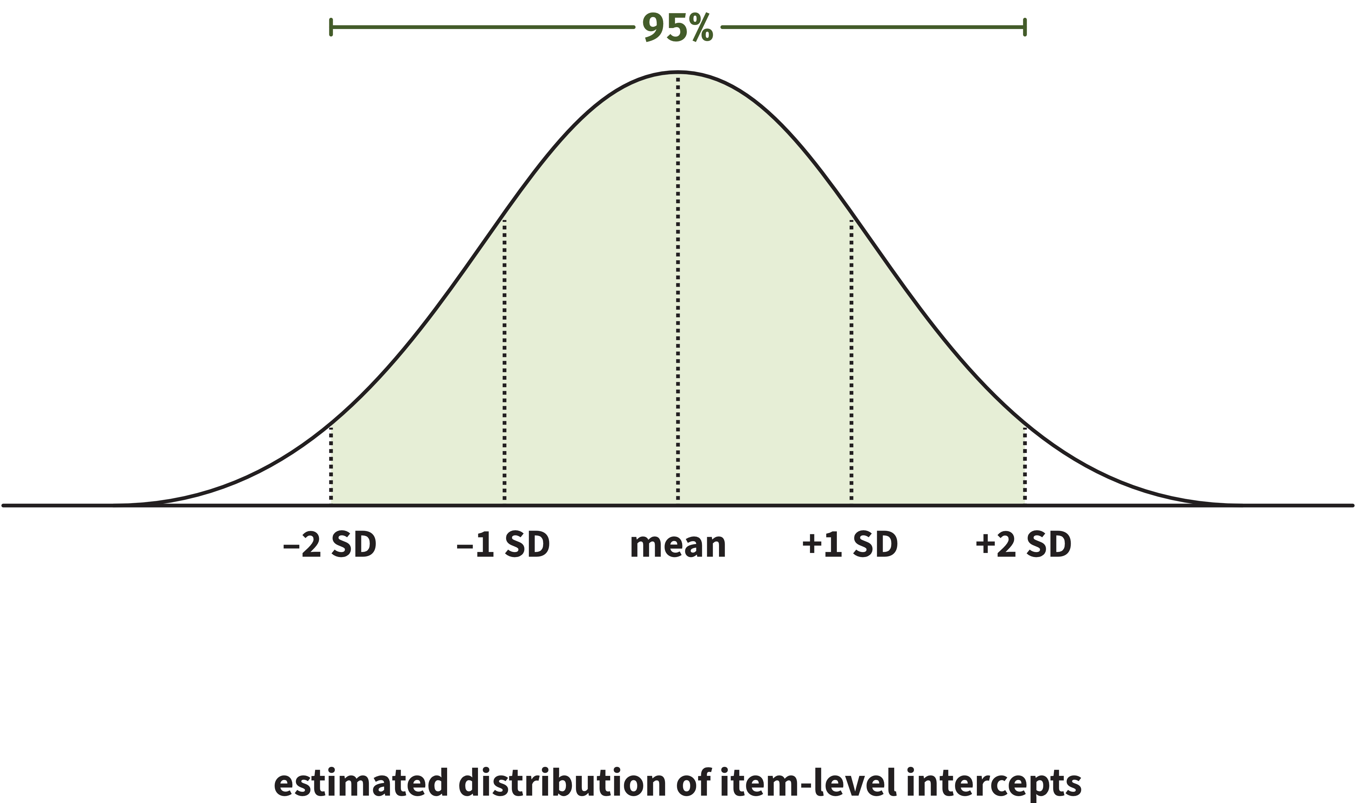
Intercept adjustments for each item_id

  Groups   Name              Variance Std.Dev. Corr 

  item_id  (Intercept)       0.7759   0.881         

Calculate the range in which the 95% of item-level intercepts are estimated to fall.

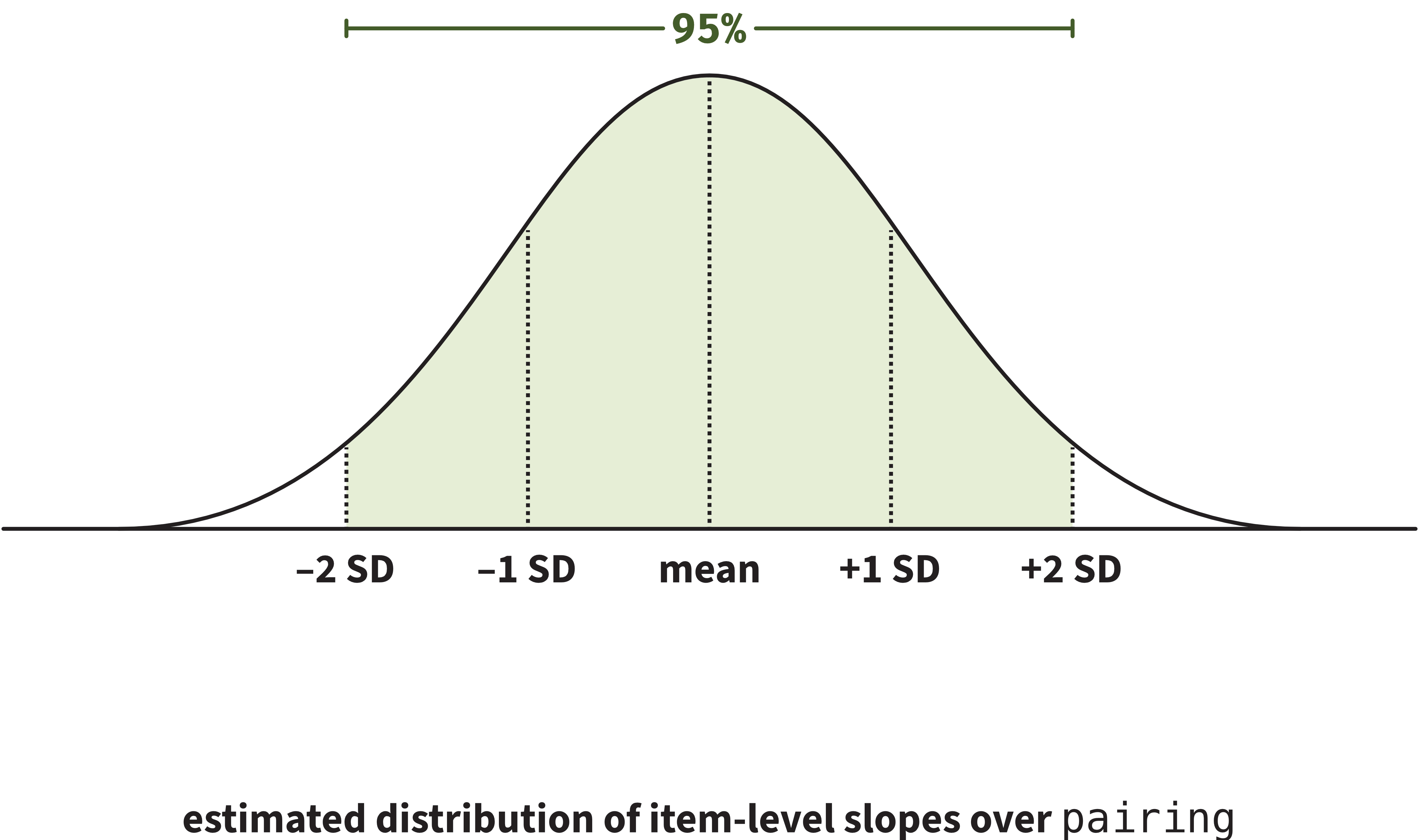
pairingAssociated adjustments for item_id

  Groups   Name              Variance Std.Dev. Corr 

  item_id  (Intercept)       0.7759   0.881         
           pairingAssociated 0.1508   0.388    -0.77

Calculate the range in which the 95% of item-level slopes over pairing are estimated to fall.

Correlation between by-item intercept and slope adjustments

  Groups   Name              Variance Std.Dev. Corr 

  item_id  (Intercept)       0.7759   0.881         
           pairingAssociated 0.1508   0.388    -0.77

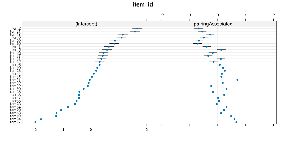
The item-level (Intercept) and pairingAssociated adjustments have a correlation of –0.77.

dotplot.ranef.mer(ranef(implicit_full_lmm))$item_id

Residuals

 Groups   Name              Variance Std.Dev. Corr 

 Residual                   0.2730   0.522         

• A residual is the difference between the value we observed for a data point and the value that the model predicts for it.

• Residuals are how the model deals with the unsystematic leftover variability that is present in the world but not accounted for by variables we’ve included in the model.

• Residual variance/SD is not very informative or useful. You don’t need to interpret or report it.

One last thing to report:
Plots of model-fitted values

Use Effect() to compute model-fitted values

In the library effects, there is a function called Effect().

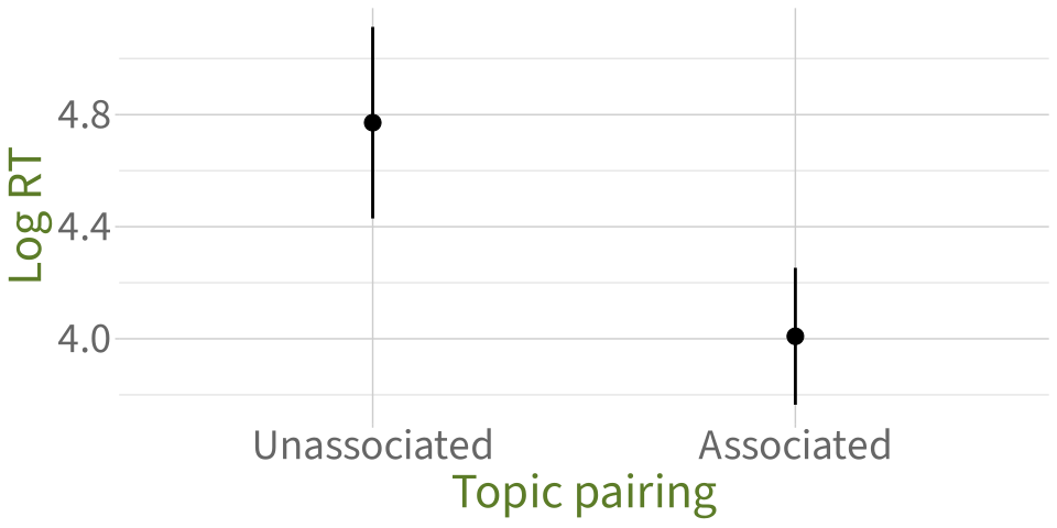
It gives us the outcome values that the model would estimate/predict for each level of our predictor, as well as the 95% CI around those values. (Same idea as emmeans from DAPR2.)

library(effects)

Effect(
  focal.predictors = c("pairing"),   # what predictor(s) do we want predictions for?
  mod = implicit_full_lmm            # what model should predictions be based on?
) |>
  as.data.frame()

       pairing  fit    se lower upper
1 Unassociated 4.77 0.174  4.43  5.11
2   Associated 4.01 0.125  3.76  4.25

• fit: the estimated outcome (log RT) value for each level of pairing
• se: the standard error of that estimate
• lower: the lower bound of the estimate’s 95% CI
• upper: the upper bound of the estimate’s 95% CI

Visualise these estimates

Effect(focal.predictors = c("pairing"), mod = implicit_full_lmm) |>
  as.data.frame() |>
  ggplot(aes(x = pairing, y = fit)) +
  geom_point() +
  geom_errorbar(aes(ymin = lower, ymax = upper), width = 0) +
  labs(
    y = 'Log RT',
    x = 'Topic pairing'
  )

How to identify all possible random effects

How to identify all possible random effects

Four steps that you can apply to any dataset + RQ:

1. Use your RQ to figure out what your model’s outcome and predictors are (i.e., your model’s fixed effects).

2. For all variables that are not the outcome or predictors, identify whether they are grouping variables.

3. Identify which of those grouping variables contribute random / non-manipulated / non-controlled variability to your data (think about the data generating process).

For every randomly-varying grouping variable, your model must contain a random intercept for that grouping variable.

4. Refer back to all predictors you identified in Step 1. For each randomly-varying grouping variable, check whether the predictor varies within that grouping variable. (To do that, check whether at least some levels of the grouping variable appear with more than one value of the predictor.)

If they do, then (in addition to the random intercepts) your model can also contain a random slope over that predictor for that grouping variable.

If they don’t, then a random slope over that predictor is impossible.

Example 1: Hesitation markers and believability

Example 1: Hesitation markers and believability

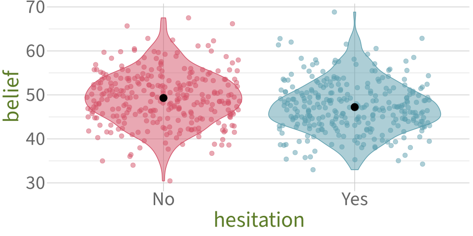
RQ: Do hesitation markers like “um”/“erm” affect how believable true statements seem?

Examples from condition hesitation = No:

• “A hashtag is technically called an octothorp.”
• “The largest snowflake was bigger than most pizzas.”
• “Pigs don’t sweat.”

Examples from condition hesitation = Yes:

• “Erm … a hashtag is technically called an octothorp.”
• “Erm … the largest snowflake was bigger than most pizzas.”
• “Erm … pigs don’t sweat.”

belief_data |>
  ggplot(aes(x = hesitation, y = belief, colour = hesitation, fill = hesitation)) +
  geom_violin(alpha = 0.5) +
  geom_jitter(alpha = 0.5, size = 3) +
  stat_summary(geom = 'point', fun = mean, colour = 'black', size = 5) +
  scale_fill_manual(values = pal) +
  scale_colour_manual(values = pal) +
  theme(
    legend.position = 'none'
  )

The data

belief_data |> head(20)

# A tibble: 20 x 5
   ppt   sentence statement                                    hesitation belief
   <chr>    <dbl> <chr>                                        <fct>       <dbl>
 1 ppt_1        1 Candy floss was invented by a dentist        Yes          53.2
 2 ppt_1        2 The first speeding fine was given in 1896    Yes          44.7
 3 ppt_1        3 Honey doesn't go off                         Yes          46.9
 4 ppt_1        4 A dog was voted mayor of a town in Minnesot~ Yes          50.8
 5 ppt_1        5 The largest snowflake was bigger than most ~ Yes          44.5
 6 ppt_1        6 Water makes different sounds depending on i~ Yes          55.9
 7 ppt_1        7 Mickey Mouse was originally called Mortimer  Yes          44.0
 8 ppt_1        8 Cats have 5 paws on their front feet and 4 ~ Yes          49.0
 9 ppt_1        9 It's impossible to hum while holding your n~ Yes          45.2
10 ppt_1       10 You can draw a line 35 miles long using one~ Yes          48.8
11 ppt_1       11 The Sahara desert is only 25% sand           No           53.6
12 ppt_1       12 A hashtag is technically called an octothorp No           42.4
13 ppt_1       13 It would take 19 minutes to fall to the cen~ No           52.2
14 ppt_1       14 Sloths don't fart                            No           55.0
15 ppt_1       15 Pigs don't sweat                             No           46.7
16 ppt_1       16 The Eiffel Tower grows 6 inches in summer    No           51.9
17 ppt_1       17 Flamingos are pink because of their diet     No           44.2
18 ppt_1       18 Rabbits can't be sick                        No           50.5
19 ppt_1       19 The dot over a lowercase i and j is called ~ No           36.4
20 ppt_1       20 The square root of 16 is 4                   No           59.7

Step 1: Identify fixed effects

1. Use your RQ to figure out what your model’s outcome and predictors are (i.e., your model’s fixed effects).

RQ: Do hesitation markers like “um”/“erm” affect how believable true statements seem?

names(belief_data)

[1] "ppt"        "sentence"   "statement"  "hesitation" "belief"    

• Outcome variable: belief
• Predictor variable: hesitation

The fixed effects part of the model formula will be belief ~ hesitation.

Step 2: Identify grouping variables

2. For all variables that are not the outcome or predictors, identify whether they are grouping variables.

For ppt:

belief_data |>
  group_by(ppt) |>
  count()

 # A tibble: 30 x 2
 # Groups:   ppt [30]
    ppt        n
    <chr>  <int>
  1 ppt_1     20
  2 ppt_10    20
  3 ppt_11    20
  4 ppt_12    20
  5 ppt_13    20
  6 ppt_14    20
  7 ppt_15    20
  8 ppt_16    20
  9 ppt_17    20
 10 ppt_18    20

...

Each value of ppt appears more than once. ppt is a grouping variable   ✅

For sentence (which numbers each statement):

belief_data |>
  group_by(sentence) |>
  count()

 # A tibble: 20 x 2
 # Groups:   sentence [20]
    sentence     n
       <dbl> <int>
  1        1    30
  2        2    30
  3        3    30
  4        4    30
  5        5    30
  6        6    30
  7        7    30
  8        8    30
  9        9    30
 10       10    30

...

Each value of sentence appears more than once. sentence is a grouping variable   ✅

Step 3: Random intercepts

3. Identify which of those grouping variables contribute random / non-manipulated / non-controlled variability to your data (think about the data generating process).

For every randomly-varying grouping variable, your model must contain a random intercept for that grouping variable.

ppt:

• The RQ doesn’t specify that we manipulate or control for specific people.
• If we re-ran the study, we could recruit different participants and still address the RQ.
• We want our results to generalise across different people.
• Therefore: ppt contributes random variability, and our model needs at least a random intercept by participant.

sentence:

• The RQ doesn’t specify that we manipulate or control for specific sentences.
• If we re-ran the study, we could show people different sentences and still address the RQ.
• We want our results to generalise across different sentences.
• Therefore: sentence contributes random variability, and our model needs at least a random intercept by sentence.

The minimum LMM formula now: belief ~ hesitation + (1 | ppt) + (1 | sentence)

Step 4: Random slopes

4. Refer back to all predictors you identified in Step 1. For each randomly-varying grouping variable, check whether the predictor varies within that grouping variable. (To do that, check whether at least some levels of the grouping variable appear with more than one value of the predictor.)

If they do, then (in addition to the random intercepts) your model can also contain a random slope over that predictor for that grouping variable.

If they don’t, then a random slope over that predictor is impossible.

Do at least some levels of ppt appear with more than one value of hesitation?

stats::xtabs(
  ~ ppt + hesitation, 
  data = belief_data
)

        hesitation
 ppt      No Yes
   ppt_1  10  10
   ppt_10 10  10
   ppt_11 10  10
   ppt_12 10  10
   ppt_13 10  10
   ppt_14 10  10

...

Yes! So (1 + hesitation | ppt) is possible.

Do at least some levels of sentence appear with more than one value of hesitation?

stats::xtabs(
  ~ sentence + hesitation, 
  data = belief_data
)

        hesitation
 sentence No Yes
       1  15  15
       2  15  15
       3  15  15
       4  15  15
       5  15  15
       6  15  15

...

Yes! So (1 + hesitation | sentence) is possible.

The model with all possible random effects

belief ~ hesitation + (1 + hesitation | ppt) + (1 + hesitation | sentence)

There’s a specific name for the version of the model that has all possible random effects permitted by the data structure and the RQ.

We call it the “maximal model”.

What questions do you have right now?

Example 2: Test-enhanced learning

Example 2: Test-enhanced learning

Two groups of participants learn some new material.

One group studied the material twice (the StudyStudy group), and the other group studied the material once and then tested themselves on it (the StudyTest group).

Recall was tested immediately (one minute) after the learning session and again one week later. Time of testing is recorded in the variable Delay.

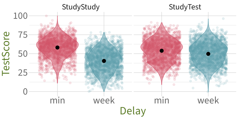
RQ: Does self-testing improve retention, such that the StudyStudy group may perform better on the immediate test, but the StudyTest group will perform better on the test one week later?

tel_data |>
  ggplot(aes(x = Delay, y = TestScore, colour = Delay, fill = Delay)) +
  geom_violin(alpha = 0.5) +
  geom_jitter(alpha = 0.15, size = 3) +
  facet_wrap(~ Group) +
  stat_summary(geom = 'point', fun = mean, colour = 'black', size = 5) +
  scale_fill_manual(values = pal) +
  scale_colour_manual(values = pal) +
  theme(
    legend.position = 'none',
    strip.background = element_blank(),
    strip.text.x = element_text(size = 24)
  )

The data

tel_data |> head(20)

# A tibble: 20 x 5
   Subject_ID  Group     Delay Test_word    TestScore
   <chr>       <chr>     <chr> <chr>            <dbl>
 1 StudyTest_A StudyTest week  carrot              52
 2 StudyTest_A StudyTest week  cane                60
 3 StudyTest_A StudyTest min   scale               54
 4 StudyTest_A StudyTest min   letter              79
 5 StudyTest_A StudyTest week  cannon              62
 6 StudyTest_A StudyTest week  pencil              30
 7 StudyTest_A StudyTest week  piano               63
 8 StudyTest_A StudyTest week  chimney             46
 9 StudyTest_A StudyTest week  pen                 64
10 StudyTest_A StudyTest week  fireplace           35
11 StudyTest_A StudyTest week  fan                 74
12 StudyTest_A StudyTest week  can                 62
13 StudyTest_A StudyTest week  fireman             52
14 StudyTest_A StudyTest min   knife               40
15 StudyTest_A StudyTest min   lamp                74
16 StudyTest_A StudyTest min   leaf                62
17 StudyTest_A StudyTest week  ring                58
18 StudyTest_A StudyTest week  cheerleaders        48
19 StudyTest_A StudyTest min   saw                 71
20 StudyTest_A StudyTest week  chair               65

Step 1: Identify fixed effects

1. Use your RQ to figure out what your model’s outcome and predictors are (i.e., your model’s fixed effects).

RQ: Does self-testing improve retention, such that the StudyStudy group may perform better on the immediate test, but the StudyTest group will perform better on the test one week later?

names(tel_data)

[1] "Subject_ID" "Group"      "Delay"      "Test_word"  "TestScore" 

• Outcome variable: TestScore
• Predictor variables: Delay, Group, and their interaction

The fixed effects part of the model formula will be TestScore ~ Delay * Group.

Step 2: Identify grouping variables

2. For all variables that are not the outcome or predictors, identify whether they are grouping variables.

The remaining variables: Subject_ID (categorical) and Test_word (categorical).

For Subject_ID:

tel_data |>
  group_by(Subject_ID) |>
  count()

 # A tibble: 20 x 2
 # Groups:   Subject_ID [20]
    Subject_ID       n
    <chr>        <int>
  1 StudyStudy_A   347
  2 StudyStudy_B   348
  3 StudyStudy_C   348
  4 StudyStudy_D   348
  5 StudyStudy_E   348
  6 StudyStudy_F   348

...

Each value of Subject_ID appears more than once. Subject_ID is a grouping variable   ✅

For Test_word:

tel_data |>
  group_by(Test_word) |>
  count()

 # A tibble: 174 x 2
 # Groups:   Test_word [174]
    Test_word     n
    <chr>     <int>
  1 ambulance    40
  2 anchor       40
  3 apple        40
  4 baby         40
  5 ball         40
  6 balloon      40

...

Each value of Test_word appears more than once. Test_word is a grouping variable   ✅

Step 3: Random intercepts

3. Identify which of those grouping variables contribute random / non-manipulated / non-controlled variability to your data (think about the data generating process).

For every randomly-varying grouping variable, your model must contain a random intercept for that grouping variable.

Subject_ID:

• The RQ doesn’t specify that we manipulate or control for specific people.
• If we re-ran the study, we could recruit different subjects and still address the RQ.
• We want our results to generalise across different people.
• Therefore: Subject_ID contributes random variability, and our model needs at least a random intercept by subject.

Test_word:

• The RQ doesn’t specify that we manipulate or control for specific test words.
• If we re-ran the study, we could show people different test words and still address the RQ.
• We want our results to generalise across different test words.
• Therefore: Test_word contributes random variability, and our model needs at least a random intercept by test word.

Minimum model now: TestScore ~ Delay * Group + (1 | Subject_ID) + (1 | Test_word)

Step 4: Random slopes

4. Refer back to all predictors you identified in Step 1. For each randomly-varying grouping variable, check whether the predictor varies within that grouping variable. (To do that, check whether at least some levels of the grouping variable appear with more than one value of the predictor.)

If they do, then (in addition to the random intercepts) your model can also contain a random slope over that predictor for that grouping variable.

If they don’t, then a random slope over that predictor is impossible.

We’ll need to check all combinations of grouping variables and predictors:

• Do at least some levels of Subject_ID appear with more than one value of Delay?
• Do at least some levels of Subject_ID appear with more than one value of Group?
• Do at least some levels of Test_word appear with more than one value of Delay?
• Do at least some levels of Test_word appear with more than one value of Group?

Step 4: Random slopes by Subject_ID

Do at least some levels of Subject_ID appear with more than one value of Delay?

stats::xtabs(
  ~ Subject_ID + Delay, 
  data = tel_data
)

              Delay
 Subject_ID     min week
   StudyStudy_A 173  174
   StudyStudy_B 174  174
   StudyStudy_C 174  174
   StudyStudy_D 174  174
   StudyStudy_E 174  174
   StudyStudy_F 174  174
   StudyStudy_G 174  174
   StudyStudy_H 174  174
   StudyStudy_I 174  174
   StudyStudy_J 174  174

...

Yes! So a random slope over Delay by Subject_ID is possible.

Do at least some levels of Subject_ID appear with more than one value of Group?

stats::xtabs(
  ~ Subject_ID + Group, 
  data = tel_data
)

              Group
 Subject_ID     StudyStudy StudyTest
   StudyStudy_A        347         0
   StudyStudy_B        348         0
   StudyStudy_C        348         0
   StudyStudy_D        348         0
   StudyStudy_E        348         0
   StudyStudy_F        348         0
   StudyStudy_G        348         0
   StudyStudy_H        348         0
   StudyStudy_I        348         0
   StudyStudy_J        348         0

...

No! People are either in one group or the other. We cannot include a random slope over Group by Subject_ID.

The maximal random effects term for Subject_ID is (1 + Delay | Subject_ID).

Step 4: Random slopes by Test_word

Do at least some levels of Test_word appear with more than one value of Delay?

stats::xtabs(
  ~ Test_word + Delay, 
  data = tel_data
)

              Delay
 Test_word      min week
   ambulance     20   20
   anchor        20   20
   apple         20   20
   baby          20   20
   ball          20   20
   balloon       20   20
   banana        20   20
   basket        20   20
   bat           20   20
   beard         20   20

...

Yes! So a random slope over Delay by Test_word is possible.

Do at least some levels of Test_word appear with more than one value of Group?

stats::xtabs(
  ~ Test_word + Group, 
  data = tel_data
)

              Group
 Test_word      StudyStudy StudyTest
   ambulance            20        20
   anchor               20        20
   apple                20        20
   baby                 20        20
   ball                 20        20
   balloon              20        20
   banana               20        20
   basket               20        20
   bat                  20        20
   beard                20        20

...

Yes! So we can also add on a random slope over Group by Test_word.

And because both predictors can have random slopes, we can also include their interaction.

The maximal random effects term for Test_word is (1 + Delay * Group | Test_word).

The maximal model

TestScore ~ Delay * Group + (1 + Delay | Subject_ID) + (1 + Delay * Group | Test_word)

Why is it useful to find the maximal model?

Why is it useful to find the maximal model?

Because the maximal model …

• … takes into account all the variability that plays a role in our design.
• … gives us the most conservative fixed effect estimates, which lowers the risk of Type I error (that is, rejecting the H0 when there is no effect).
• … generalises better to the populations that we want to draw conclusions about.

From a theoretical perspective, the maximal model is what we should fit. But from a practical perspective, sometimes this is actually impossible to do in R.

For example, take the maximal model for our RQ for tel_data:

TestScore ~ Delay * Group + (1 + Delay | Subject_ID) + (1 + Delay * Group | Test_word)

If we try to fit this model, R will not be able to do it.

Next week, we’ll learn how to deal with that issue.

Regardless of any practical issues that happen when we try to fit the model, we should always start an analysis by finding the maximal model permitted by our dataset and RQ.

What questions do you have right now?

Back matter

Learning objectives revisited

How do we interpret the random effects part of a model summary?

• Always relative to the fixed effects.
• The fixed effect is the mean of a Normal distribution of group-level adjustments.
• The SD of that Normal distribution is given in the random effects summary table.
• There is no significance testing involved for random effects.
• When interpreting random effects, we are interested in questions like:
  • Is there greater variability within one grouping variable than another?
  • For slope adjustments: does the model predict that any specific levels of the grouping variable show the opposite direction of effect (e.g., a negative effect if the fixed effect is positive)?

How do we know if a model can include random intercepts for a given grouping variable?

• We think about the data generating process, and specifically the kind of variability that the grouping variable contributes to the data.
• If the grouping variable contributes random variability to the data, then a model of that data must include random intercepts for that grouping variable.

Learning objectives revisited

How do we know if a model can include random slopes over a given predictor for a given grouping variable?

• Check if the data contains more than one value of a given predictor within at least some levels of the grouping variable.
• (Why? Because we need at least two observations to fit a line. If there’s only one value for a given predictor and a given participant, then we have no idea what a line fit to that data would look like because we don’t know the second point that the line would connect.)

What is a maximal model?

• A model that contains all possible random effects that are permitted by the data structure and the RQ.

To do this week

Tasks:

Work on exercises in labs

Complete the weekly quiz

Get support:

Consult the flash cards

Ask questions anonymously on Piazza

We really like seeing you in office hours!

Intercepts

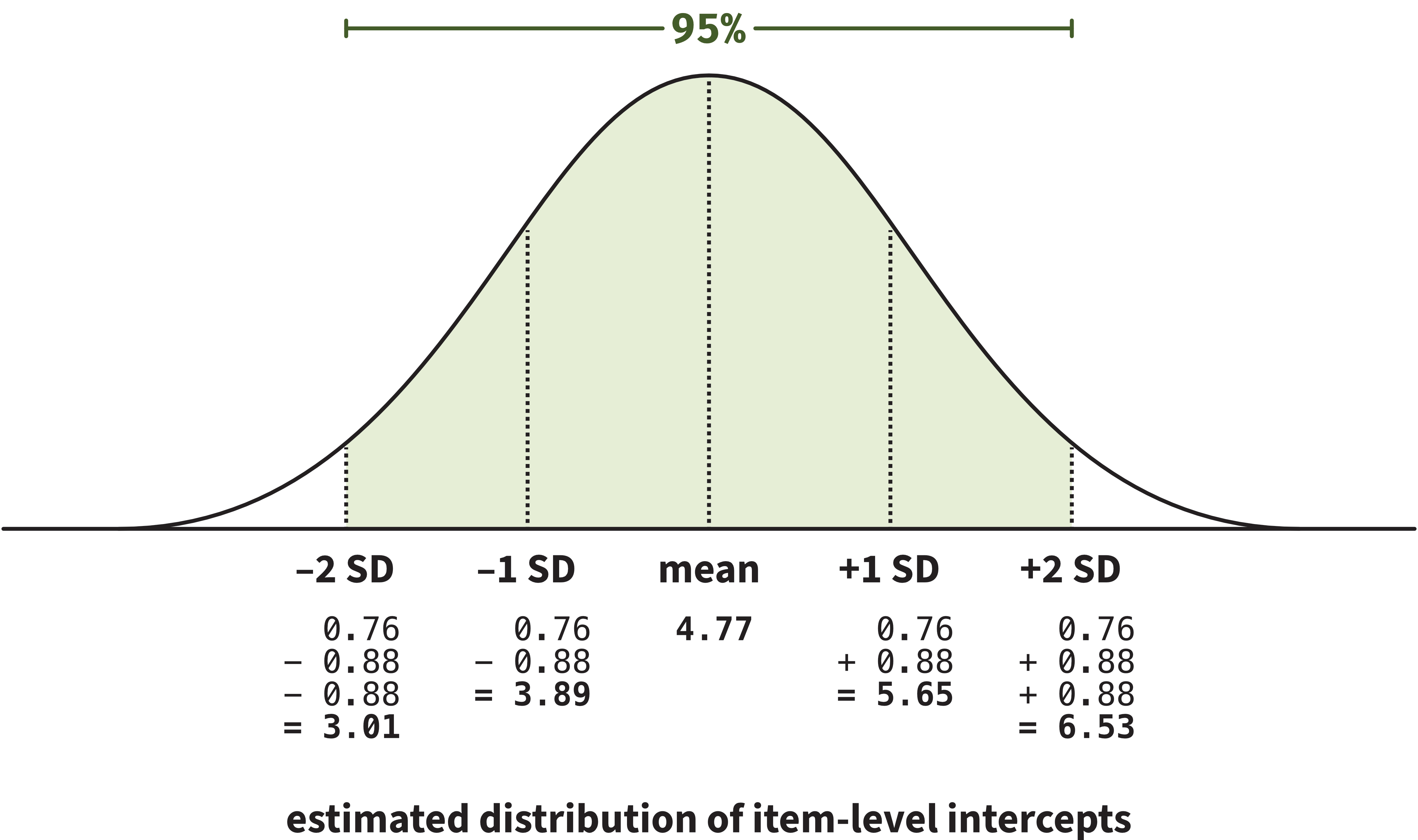
• 95% of item-level intercepts are estimated to fall between about 3.01 log units and 6.53 log units.

• For 95% of items, the estimated log RT when the item is seen as part of an unassociated pairing is between 3.01 log units and 6.53 log units.

• This range for items is larger than the range for participants, which means that items show more variability around the fixed intercept than participants do.

Slopes

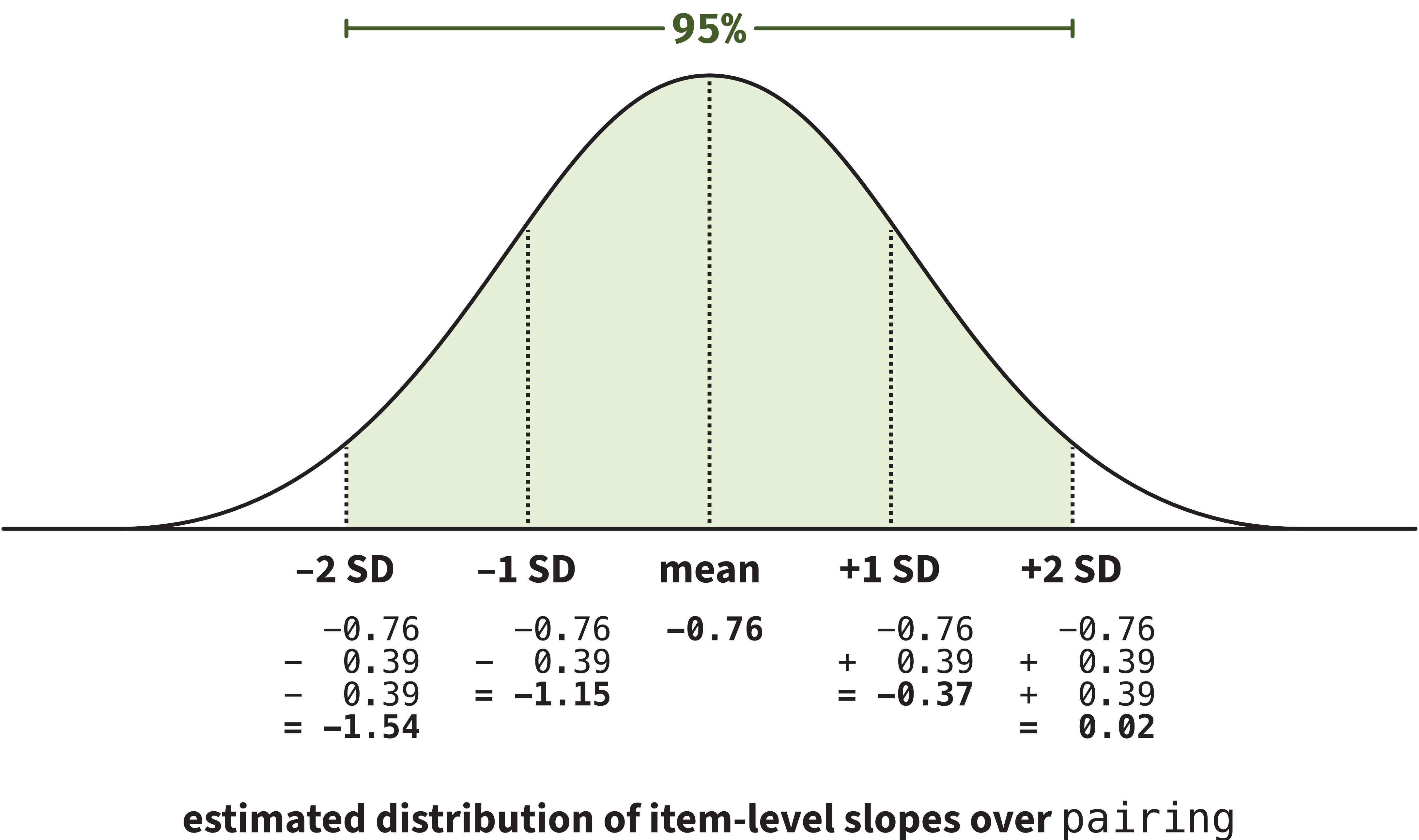
• 95% of item-level slopes over pairing are estimated to fall between about –1.54 log units and 0.02 log units.

• This is interesting because some items appear to show a tiny positive effect of pairing! In other words, they might elicit faster reactions for unassociated pairings and slower reactions for associated pairings—not the pattern we expected.

• Useful information!!