|
Linear mixed models (with Dr. Elizabeth Pankratz) |
Regression refresher, intro to group-structured data |
| Modelling group-structured data using random effects | |
| Interpreting LMMs and building maximal models | |
| Troubleshooting model fit, checking assumptions + diagnostics | |
| LMMs: Practice analysis | |
|
factor analysis working with multi-item measures (with Dr. Josiah King) |
measurement and dimensionality |
| exploring underlying constructs (EFA) | |
| testing theoretical models (CFA) | |
| reliability and validity | |
| recap & exam prep |
Regression refresher,
intro to group-structured data
Data Analysis for Psychology in R 3
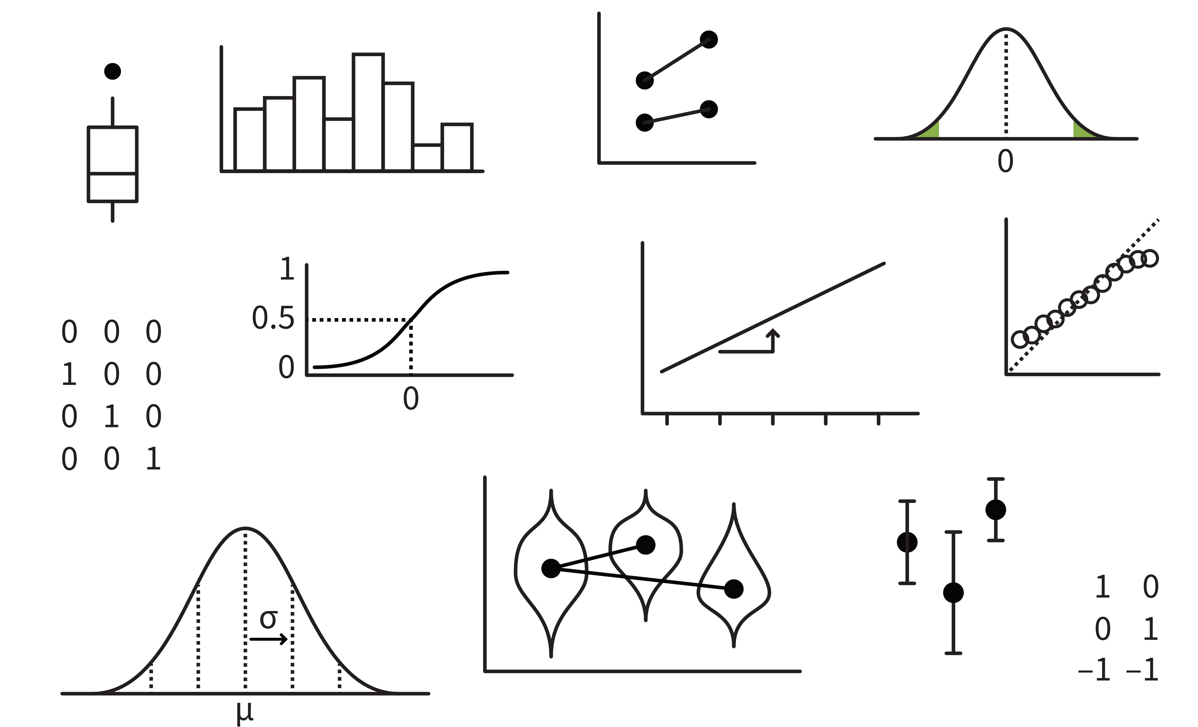
Part 1: Brain dump all the stats terms you know/remember
Here are some visuals that might help jog your memory:
Part 2: Connect key ideas
Example terms:
- standard deviation (SD)
- standard error (SE)
- confidence interval (CI)
Individually or with your seatmates:
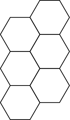
- Relax while Elizabeth transfers key terms to the hexagon sheet
- Using a big-screened device, access hexagons at this link: https://edin.ac/4cQpsUM
- Duplicate Slide 1 and work on your own duplicated copy
- Click and drag each term from the menu onto its own hexagon. If two hexagons are touching, then the ideas on each hexagon are somehow connected.
There are no wrong answers here! The purpose of this activity is to help you remember a few of the ways that a few big ideas fit together.
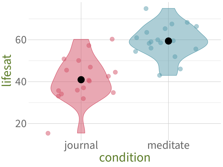
Data: After one week of mindfulness treatments, life satisfaction ratings from 36 people
Code
set.seed(1)
p_lifesat <- lifesat |>
  ggplot(aes(x = condition, y = lifesat, fill = condition, colour = condition)) +
  geom_violin(alpha = 0.5) +
  geom_jitter(alpha = 0.5, size = 5) +
  stat_summary(geom = 'point', fun = mean, colour = 'black', size = 8) +
  theme(legend.position = 'none') +
  scale_colour_manual(values = pal) +
  scale_fill_manual(values = pal) +
  NULL
p_lifesat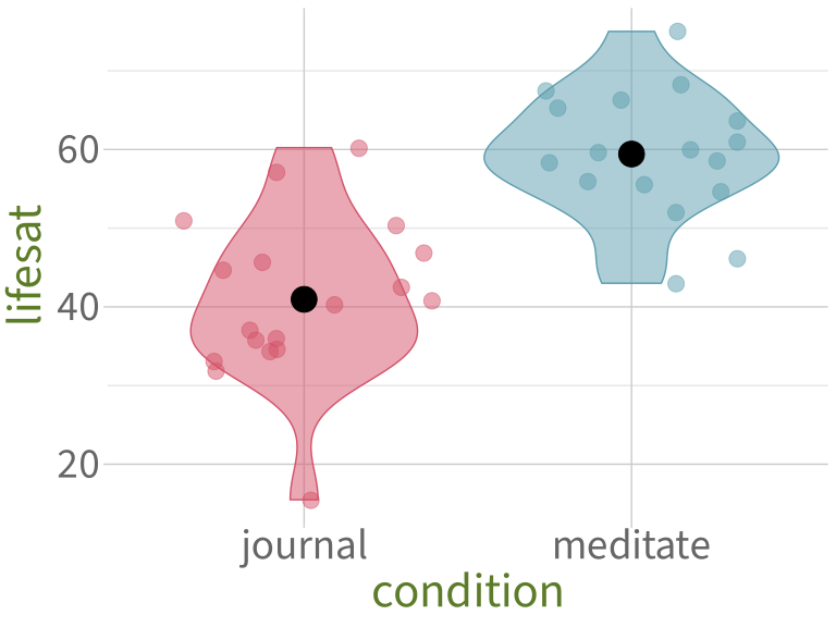
lifesat |>
  head(15)
# A tibble: 15 x 3
condition ppt_id lifesat
<chr> <chr> <dbl>
1 journal j1 34.2
2 journal j2 42.5
3 journal j3 45.6
4 journal j4 44.6
5 journal j5 35.7
6 journal j6 50.2
7 journal j7 31.9
8 journal j8 40.7
9 journal j9 57.2
10 journal j10 37.0
11 journal j11 33.0
12 journal j12 46.9
13 journal j13 34.7
14 journal j14 36.1
15 journal j15 60.2Numerically, there is a difference between condition means: “meditate” has higher lifesat than “journal”.
We want to test: Is that difference between condition means sufficiently unlikely to equal zero?
Is the difference between condition means sufficiently unlikely to equal zero?
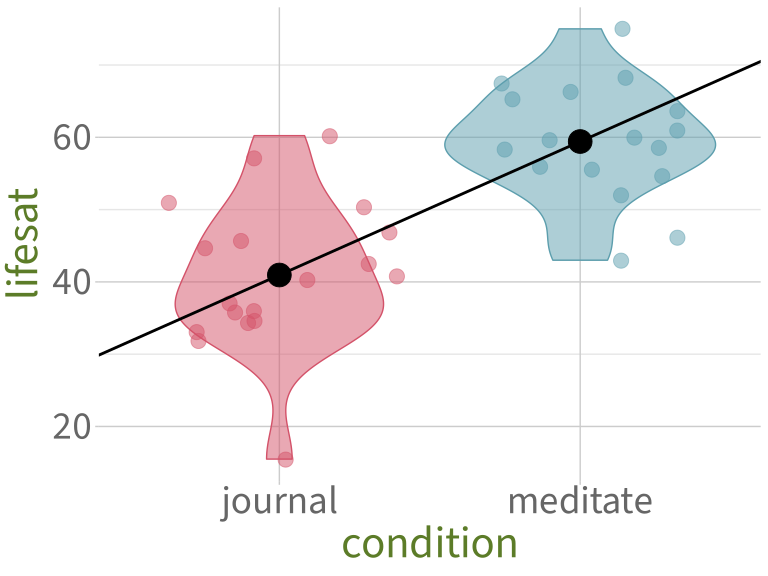
A linear model will fit a line that passes through the two group means.
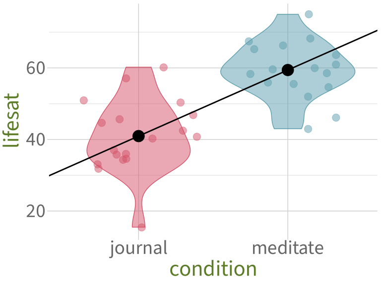
To answer our question, we will first imagine that in reality, the true slope of this line is zero: the groups are not different at all (= our null hypothesis).
In that reality where the groups are not different, we know the distribution of values that the slope could reasonably have.
We compare that null distribution to the slope we have actually observed.
If our observed slope falls in either tail of the null distribution, then we can say that the slope is significantly different from zero!
Interpret model coefficients
Coefficients:
                   Estimate Std. Error t value   Pr(>|t|)
 (Intercept)          40.95       2.17   18.88    < 2e-16 ***
 conditionmeditate    18.47       3.07    6.02 0.00000081 ***
(Intercept) = the estimated average lifesat for condition = 0, the reference level, which is journal.
- People who journal are estimated to have a life satisfaction of 40.95 points, on average.
- This estimate is significantly different from zero (\(p\) < .001), but that’s not very surprising or interesting.
conditionmeditate: = the difference between the average lifesat when condition = 1 = meditate and the average lifesat when condition = 0 = journal.
- People who meditate are estimated to have a life satisfaction that’s 18.47 points greater than people who journal.
- This estimate is significantly different from zero (\(p\) < .001).
So yes, the difference between condition means is sufficiently unlikely to equal zero!
We reject the H0 and declare that the groups are significantly different.
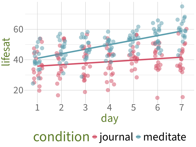
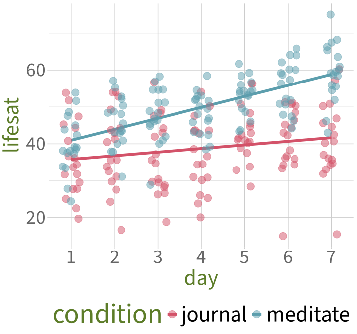
An example of repeated-measures data:
One week of mindfulness treatments
Code
p_lifesat_week <- lifesat_week |>
  ggplot(aes(x = day, y = lifesat, colour = condition)) +
  geom_smooth(method ='lm', se = F, formula = 'y ~ x', linewidth = 2) +
  geom_jitter(alpha = 0.5, width = .2, size = 5) +
  scale_colour_manual(values = pal) +
  scale_x_continuous(breaks = 1:7) +
  theme(
    legend.position = 'bottom',
    panel.grid.minor.x = element_blank()
  ) +
  NULL
p_lifesat_week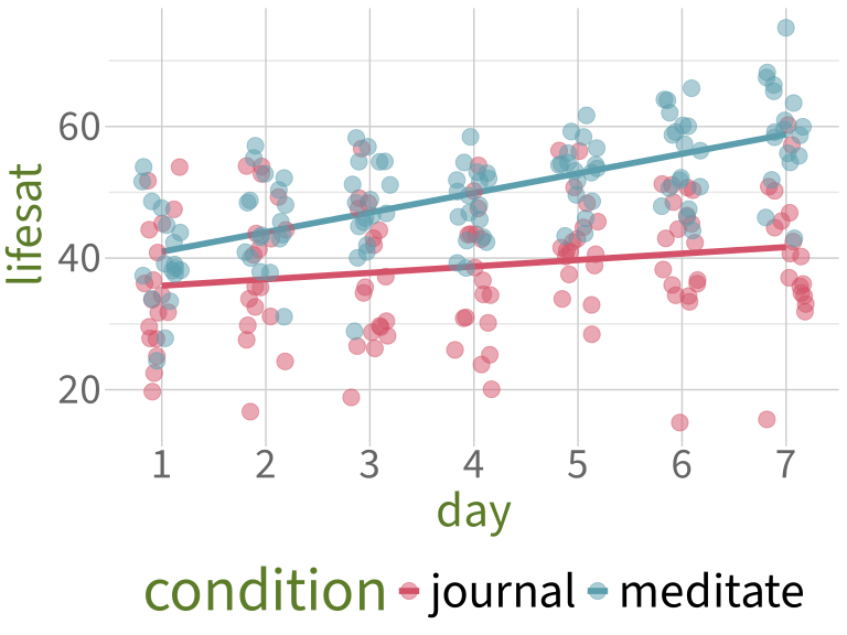
lifesat_week |>
  head(15)
# A tibble: 15 x 4
day condition ppt_id lifesat
<dbl> <chr> <chr> <dbl>
1 1 journal j1 36.6
2 2 journal j1 33.8
3 3 journal j1 44.2
4 4 journal j1 25.3
5 5 journal j1 42.4
6 6 journal j1 45.2
7 7 journal j1 34.2
8 1 journal j2 22.5
9 2 journal j2 40.5
10 3 journal j2 34.7
11 4 journal j2 43.5
12 5 journal j2 41.1
13 6 journal j2 44.4
14 7 journal j2 42.5
15 1 journal j3 51.8(In the example from before, we were looking at data from Day 7 only!)
RQs: Does life satisfaction increase, the longer people take part in treatment? Is one treatment associated with greater life satisfaction than the other?
Why aren’t the data points independent?
Code
lifesat_week |>
  filter(ppt_id %in% c('j16', 'm9')) |>
  ggplot(aes(x = day, y = lifesat, colour = ppt_id, shape = ppt_id)) +
  geom_point(size = 7) +
  scale_colour_manual(values = pal[2:3]) +
  scale_x_continuous(breaks = 1:7) +
  theme(
    legend.position = 'bottom',
    panel.grid.minor.x = element_blank()
  ) +
  NULL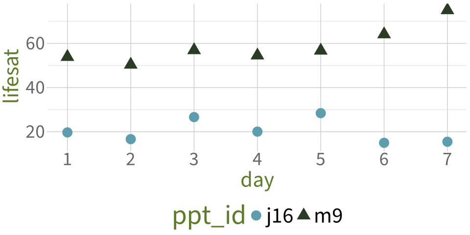
If we know one data point from m9, we can make some good guesses about what values m9’s other data points might have. Same for j16.
- In other words: Some of our data gives us information about other parts of our data.
- In other words: Data points from one person are not independent of other data points from that same person.
We use grouping variables to tell the model that data points are not independent, and instead are grouped together in this way.
- The specifics of how we tell the model about grouping variables: next week.
- This week: how we identify grouping variables in any dataset.
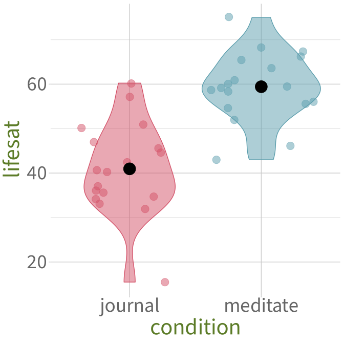
Ex. 1: Mindfulness treatments, Day 7
What categorical variables do we have in lifesat?
glimpse(lifesat)Rows: 36
Columns: 3
$ condition <chr> "journal", "journal", "journal", "journal", "journal", "jour~
$ ppt_id <chr> "j1", "j2", "j3", "j4", "j5", "j6", "j7", "j8", "j9", "j10",~
$ lifesat <dbl> 34.2, 42.5, 45.6, 44.6, 35.7, 50.2, 31.9, 40.7, 57.2, 37.0, ~Ex. 2: A week of mindfulness treatments
What categorical variables do we have in lifesat_week?
glimpse(lifesat_week)Rows: 252
Columns: 4
$ day <dbl> 1, 2, 3, 4, 5, 6, 7, 1, 2, 3, 4, 5, 6, 7, 1, 2, 3, 4, 5, 6, ~
$ condition <chr> "journal", "journal", "journal", "journal", "journal", "jour~
$ ppt_id <chr> "j1", "j1", "j1", "j1", "j1", "j1", "j1", "j2", "j2", "j2", ~
$ lifesat <dbl> 36.6, 33.8, 44.2, 25.3, 42.4, 45.2, 34.2, 22.5, 40.5, 34.7, ~Ex. 1: Mindfulness treatments, Day 7
Ex. 2: A week of mindfulness treatments
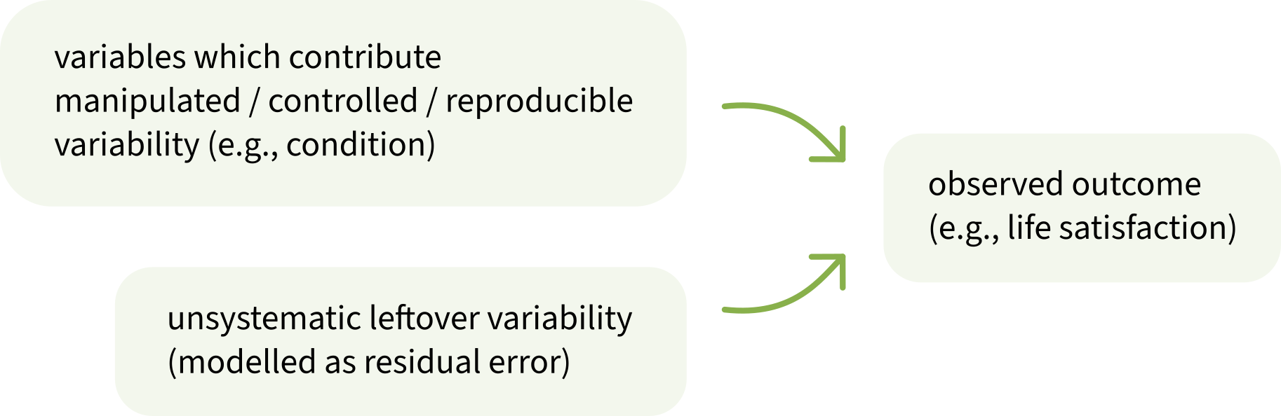
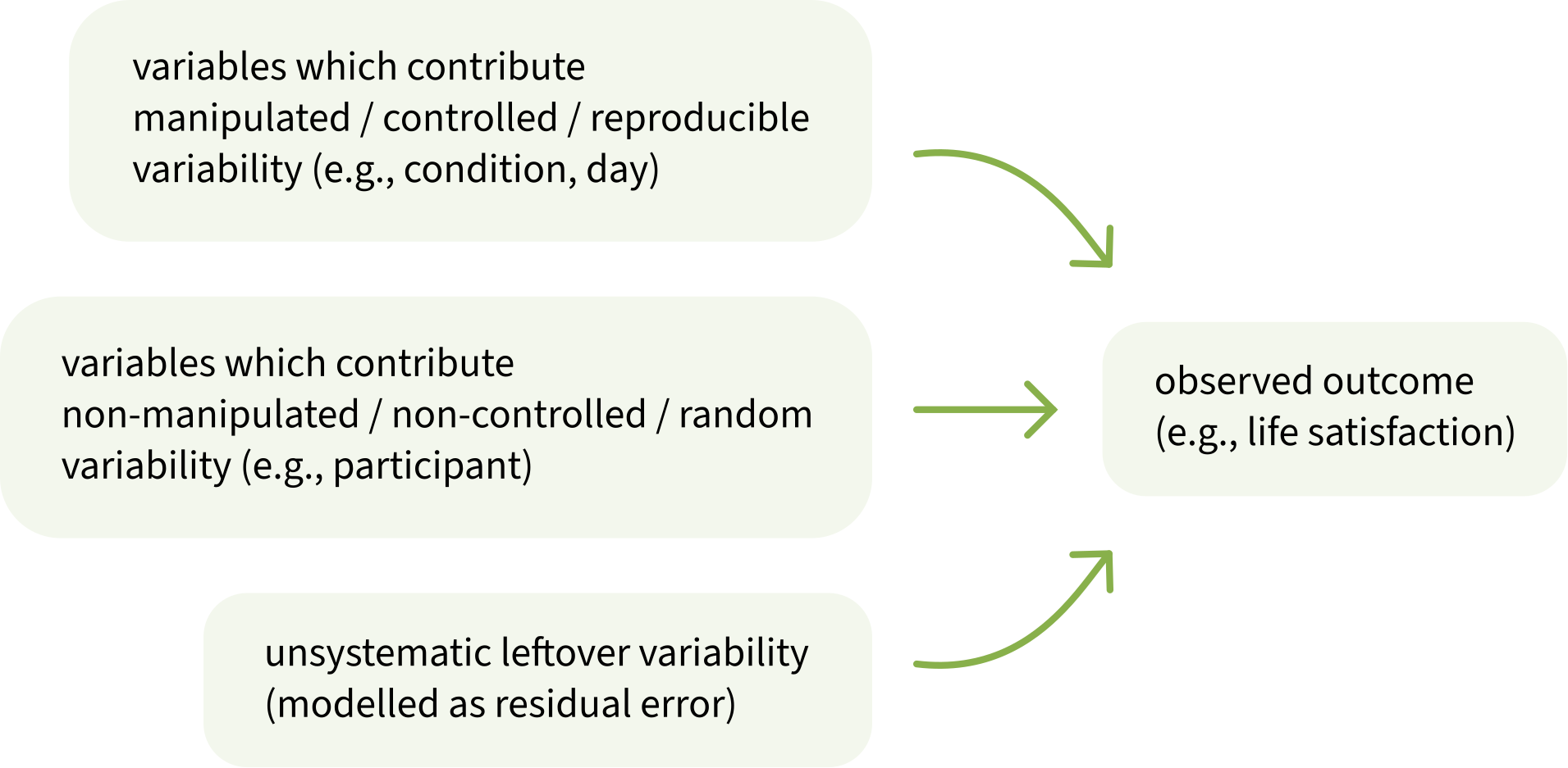
When we have multiple observations from a single source (here, a single person), we have something new: random, non-manipulated variability that comes from a specific variable.
To do this week
Tasks:
 Work on exercises in labs
 Complete the weekly quiz
Get support:
 Consult the flash cards
 Ask questions anonymously on Piazza
 We really like seeing you in office hours!
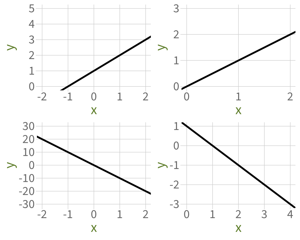
Line plots from Wooclap
Code
p1 <- ggplot() +
  geom_abline(aes(intercept = 1, slope = 1), linewidth = 2) +
  scale_x_continuous(limits = c(-2, 2), breaks = -2:2) +
  scale_y_continuous(limits = c(0, 5), breaks = 0:5) +
  theme(panel.grid.minor = element_blank()) +
  labs(x = 'x', y = 'y') +
  NULL
# ggsave('figs/woo/w1-p1.png', width = 10, height = 10, units = 'cm')

p2 <- ggplot() +
  geom_abline(aes(intercept = 0, slope = 1), linewidth = 2) +
  scale_x_continuous(limits = c(0, 2), breaks = 0:2) +
  scale_y_continuous(limits = c(0, 3), breaks = 0:3) +
  theme(panel.grid.minor = element_blank()) +
  labs(x = 'x', y = 'y') +
  NULL
# ggsave('figs/woo/w1-p2.png', width = 10, height = 10, units = 'cm')

p3 <- ggplot() +
  geom_abline(aes(intercept = 0, slope = -10), linewidth = 2) +
  scale_x_continuous(limits = c(-2, 2)) +
  scale_y_continuous(limits = c(-30, 30), breaks = seq(-30, 30, by=10)) +
  theme(panel.grid.minor = element_blank()) +
  labs(x = 'x', y = 'y') +
  NULL
# ggsave('figs/woo/w1-p3.png', width = 10, height = 10, units = 'cm')

p4 <- ggplot() +
  geom_abline(aes(intercept = 1, slope = -1), linewidth = 2) +
  scale_x_continuous(limits = c(0, 4), breaks = 0:4) +
  scale_y_continuous(limits = c(-3, 1), breaks = -3:5) +
  theme(panel.grid.minor = element_blank()) +
  labs(x = 'x', y = 'y') +
  NULL
# ggsave('figs/woo/w1-p4.png', width = 10, height = 10, units = 'cm')

p1 + p2 + p3 + p4