| person | y | x | ... |
|---|---|---|---|
| 1 | ... | ... | ... |
| 1 | ... | ... | ... |
| 1 | ... | ... | ... |
| 2 | ... | ... | ... |
| 2 | ... | ... | ... |
| 2 | ... | ... | ... |
| 3 | ... | ... | ... |
| 3 | ... | ... | ... |
| 3 | ... | ... | ... |
Recap!
Data Analysis for Psychology in R 3
things we’ve explored…
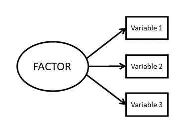
the idea
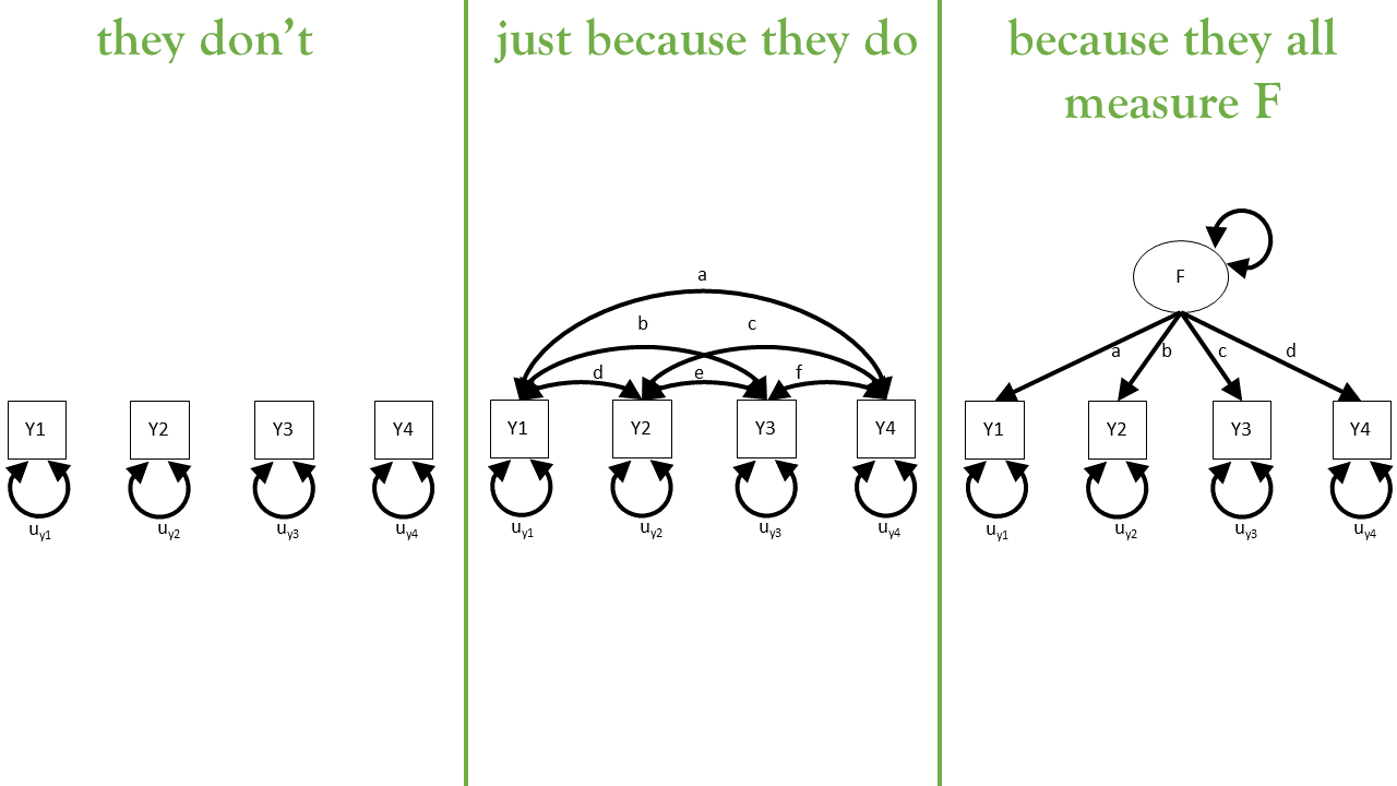
cov/cor between times can reflect the extent to which items ‘measure the same thing’
- people vary in lots of ways over k variables
- capture the ways in which people vary.

the idea
cov/cor between times can reflect the extent to which items ‘measure the same thing’
- people vary in lots of ways over k variables
- capture the ways in which people vary.

loadings - orthogonal EFA
library(psych)
fa(somedata, nfactors=2, rotate="varimax")
Factor Analysis using method = minres
Call: fa(r = somedata, nfactors = 2, rotate = "varimax")
Standardized loadings (pattern matrix) based upon correlation matrix
MR1 MR2 h2 u2 com
y1 0.84 0.25 0.78 0.22 1.2
y2 0.87 0.11 0.77 0.23 1.0
y3 0.88 0.04 0.77 0.23 1.0
y4 0.11 0.90 0.82 0.18 1.0
y5 0.16 0.81 0.69 0.31 1.1
y6 0.13 0.78 0.62 0.38 1.1
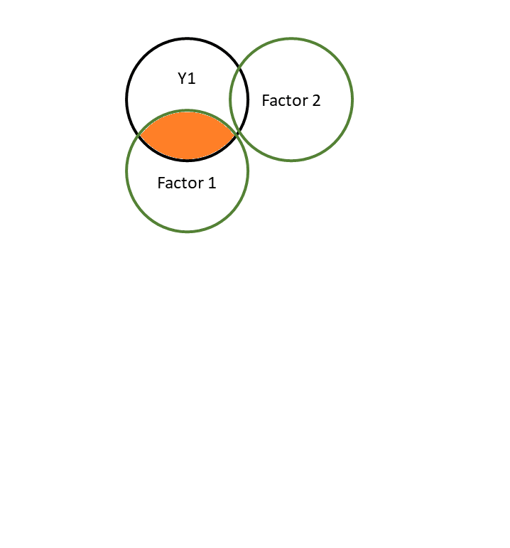
...loadings
cor(item, Factor)
lm(item ~ Factor)
(where items and Factors are standardised)
loadings\(^2\)
- variance in item explained by Factor (like \(R^2\)!)
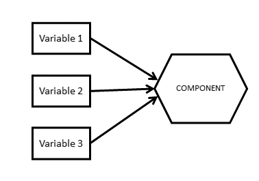
EFA compared to PCA
Pretty much the same idea: captures relations between items and dimensions, and variance explained by dimensions
BUT - the aim is to explain, not just reduce
- best explanation becomes theory driven, and is focused on having a “simple structure” (think: clearly defined dimensions).
blurred lines
in psych, PCA is often used as a type of EFA (components are interpreted meaningfully, considered as ‘explanatory’, and sometimes rotated! In most other fields, PCA is pure reduction)
loadings - orthogonal EFA
library(psych)
fa(somedata, nfactors=2, rotate="varimax")Factor Analysis using method = minres
Call: fa(r = somedata, nfactors = 2, rotate = "varimax")
Standardized loadings (pattern matrix) based upon correlation matrix
MR1 MR2 h2 u2 com
y1 0.84 0.25 0.78 0.22 1.2
y2 0.87 0.11 0.77 0.23 1.0
y3 0.88 0.04 0.77 0.23 1.0
y4 0.11 0.90 0.82 0.18 1.0
y5 0.16 0.81 0.69 0.31 1.1
y6 0.13 0.78 0.62 0.38 1.1
...loadings
cor(item, Factor)
lm(item ~ Factor)
(where items and Factors are standardised)
loadings\(^2\)
- variance in item explained by Factor (like \(R^2\)!)
SSloadings & Variance Accounted for
library(psych)
fa(somedata, nfactors=2, rotate="varimax")Factor Analysis using method = minres
Call: fa(r = somedata, nfactors = 2, rotate = "varimax")
Standardized loadings (pattern matrix) based upon correlation matrix
MR1 MR2 h2 u2 com
y1 0.84 0.25 0.78 0.22 1.2
y2 0.87 0.11 0.77 0.23 1.0
y3 0.88 0.04 0.77 0.23 1.0
y4 0.11 0.90 0.82 0.18 1.0
y5 0.16 0.81 0.69 0.31 1.1
y6 0.13 0.78 0.62 0.38 1.1
MR1 MR2
SS loadings 2.28 2.15
...SSloadings
- “sum of squared loadings”
- \(R^2\) from
lm(item1 ~ Factor)+
\(R^2\) fromlm(item2 ~ Factor)+
\(R^2\) fromlm(item3 ~ Factor)+ ….
(where items and Factors are standardised)![]()
SSloadings & Variance Accounted for
Principal Components Analysis
Call: principal(r = somedata, nfactors = 6, rotate = "none")
Standardized loadings (pattern matrix) based upon correlation matrix
    PC1   PC2   PC3   PC4   PC5   PC6 h2      u2 com
y1 0.81 -0.43 -0.28  0.10 -0.16 -0.20  1 5.6e-16 2.1
y2 0.74 -0.55  0.22 -0.17 -0.23  0.16  1 4.4e-16 2.5
y3 0.69 -0.61  0.04  0.09  0.37  0.03  1 6.7e-16 2.6
y4 0.70  0.59 -0.30  0.16 -0.01  0.20  1 4.4e-16 2.7
y5 0.71  0.53 -0.03 -0.43  0.11 -0.08  1 1.1e-15 2.7
y6 0.68  0.56  0.40  0.25 -0.03 -0.09  1 1.7e-15 3.0

                       PC1  PC2  PC3  PC4  PC5  PC6
SS loadings           3.15 1.80 0.38 0.32 0.23 0.12
Proportion Var        0.52 0.30 0.06 0.05 0.04 0.02
Cumulative Var        0.52 0.83 0.89 0.94 0.98 1.00
...
h2, u2
library(psych)
fa(somedata, nfactors=2, rotate="varimax")
Factor Analysis using method = minres
Call: fa(r = somedata, nfactors = 2, rotate = "varimax")
Standardized loadings (pattern matrix) based upon correlation matrix
MR1 MR2 h2 u2 com
y1 0.84 0.25 0.78 0.22 1.2
y2 0.87 0.11 0.77 0.23 1.0
y3 0.88 0.04 0.77 0.23 1.0
y4 0.11 0.90 0.82 0.18 1.0
y5 0.16 0.81 0.69 0.31 1.1
y6 0.13 0.78 0.62 0.38 1.1
MR1 MR2
SS loadings 2.28 2.15
Proportion Var 0.38 0.36
...Communalities (h2) & Uniqueness (u2):
h2: Variance in an item explained by all factors
u2: Unexplained variance in an item
lm(item ~ F1 + F2 + ...)
(where items and Factors are standardised)- Communality = \(R^2\)
- Uniqueness = \(1-R^2\) from
EFA output and rotations
library(psych)
fa(somedata, nfactors=2, rotate="oblimin", fm="ml")$Structure
Loadings:
ML2 ML1
y1 0.875 0.408
y2 0.877 0.203
y3 0.869 0.164
y4 0.231 0.944
y5 0.270 0.791
y6 0.232 0.760
ML2 ML1
SS loadings 2.471 2.329
Proportion Var 0.412 0.388
Cumulative Var 0.412 0.800
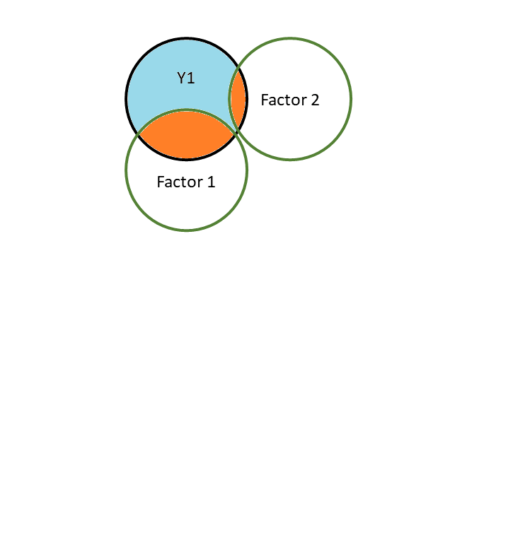
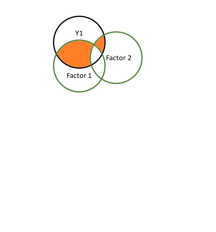
...Structure matrix
Shows
cor(item, Factor)but Factors are now correlated with one another!
EFA output and rotations
library(psych)
fa(somedata, nfactors=2, rotate="oblimin", fm="ml")$loadings
Loadings:
ML2 ML1
y1 0.826 0.178
y2 0.890 -0.045
y3 0.892 -0.084
y4 -0.035 0.953
y5 0.054 0.776
y6 0.022 0.754
ML2 ML1
SS loadings 2.275 2.120
Proportion Var 0.379 0.353
Cumulative Var 0.379 0.733
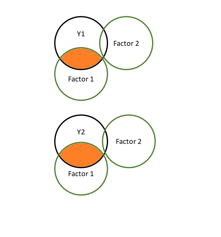
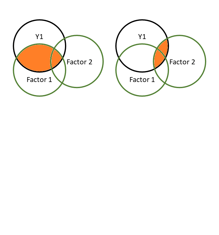
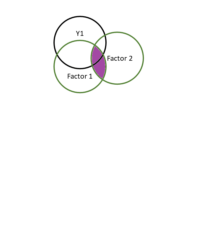
...Pattern matrix
shows variance in item uniquely explained by each Factor
like
lm(item ~ F1 + F2 + ...) |> coef()
(where items and Factors are standardised)
EFA output and rotations
library(psych)
fa(somedata, nfactors=2, rotate="oblimin", fm="ml")
Loadings:
   ML2    ML1
y1  0.826  0.178
y2  0.890 -0.045
y3  0.892 -0.084
y4 -0.035  0.953
y5  0.054  0.776
y6  0.022  0.754

                 ML2   ML1
SS loadings    2.275 2.120
Proportion Var 0.379 0.353
Cumulative Var 0.379 0.733
...
With factor correlations of ML2 ML1
ML2 1.000 0.278
ML1 0.278 1.000Factor Correlations
cor(Factor1, Factor2)
why do y1, …, y4 covary with one another?