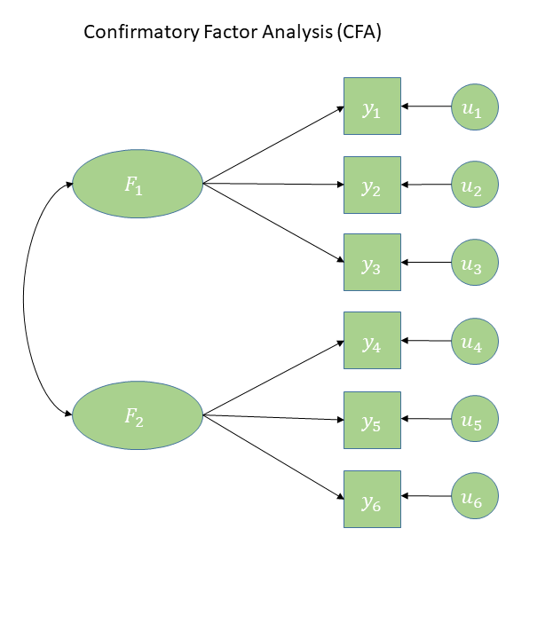
Confirmatory Factor Analysis (CFA)
Data Analysis for Psychology in R 3
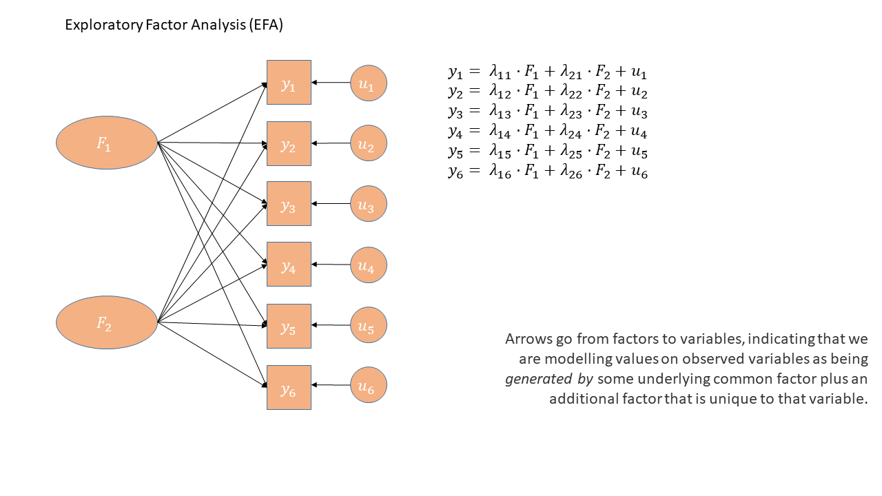
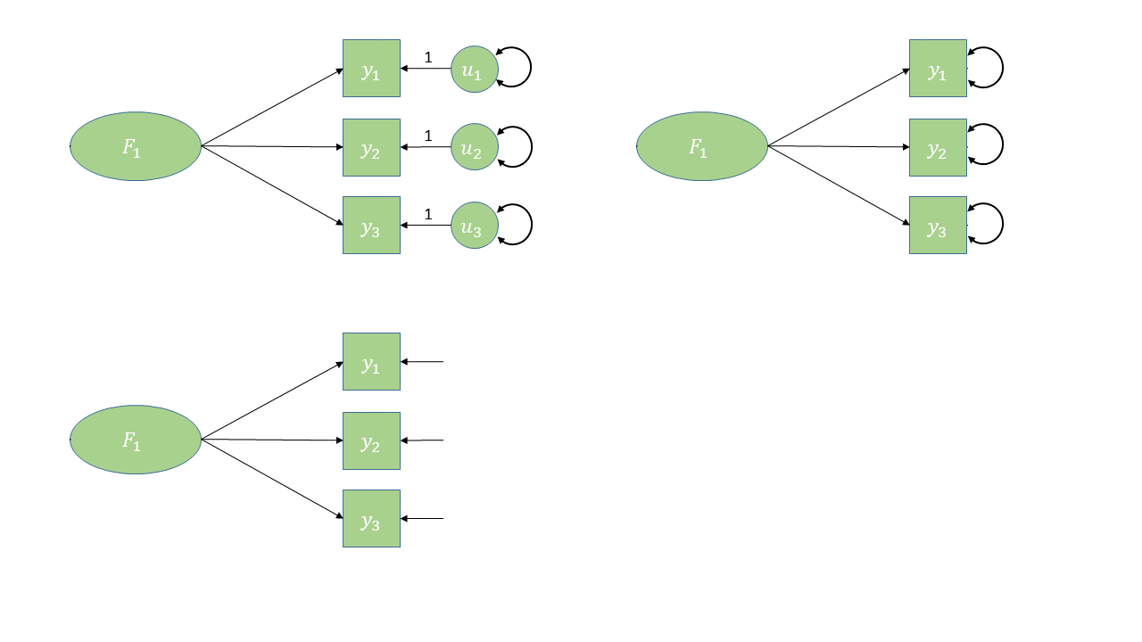
In diagrams: EFA
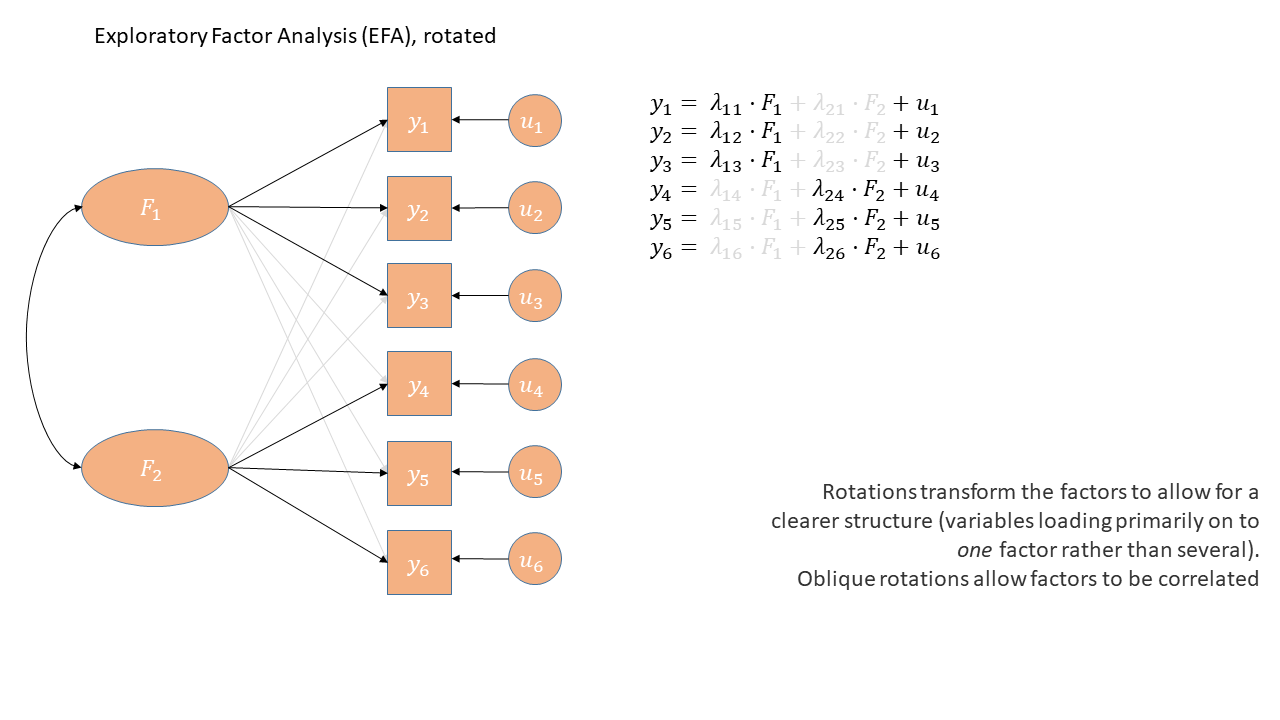
In diagrams: EFA (oblique rotation)
In diagrams: CFA
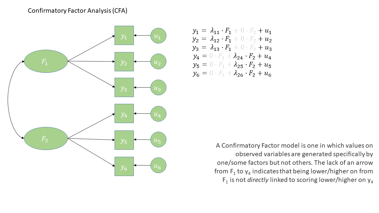
In diagrams: CFA
- Some arrows are absent
- This is what imposes our theory
- The reason that \(y_1\) and \(y_2\) are correlated is because:
- they both represent \(F_1\)
- they both represent \(F_1\)
- The reason that \(y_1\) and \(y_6\) are correlated is because:
- \(y_1\) is a manifestation of \(F_1\),
- \(y_6\) is a manifestation of \(F_2\),
- and \(F_1\) and \(F_2\) are correlated
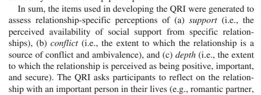
In diagrams: residuals in CFA
different ways people choose to draw the same thing…
lavaan operators
| Formula type | Operator | Mnemonic |
|---|---|---|
| latent variable definition | =~ |
“is measured by” |
| (residual) (co)variance | ~~ |
“covaries with” |
F1 =~ y1 + y2 + y3
F2 =~ y4 + y5 + y6
F1 ~~ F2
example: QRI
| var | wording |
|---|---|
| s1 | To what extent could you turn to this person for advice about problems? |
| s2 | To what extent could you count on this person for help with a problem? |
| s3 | To what extent can you really count on this person to distract you from your worries when you feel under stress? |
| s4 | To what extent can you count on this person to listen to you when you are very angry at someone else? |
| c1 | How often do you have to work hard to avoid conflict with this person? |
| c2 | How much do you argue with this person? |
| c3 | How much would you like this person to change? |
| c4 | How often does this person make you feel angry? |
| d1 | How positive a role does this person play in your life? |
| d2 | How significant is this relationship in your life? |
| d3 | How close will your relationship be with this person in 10 years? |
| d4 | How much would you miss this person if the two of you could not see or talk with each other for a month? |
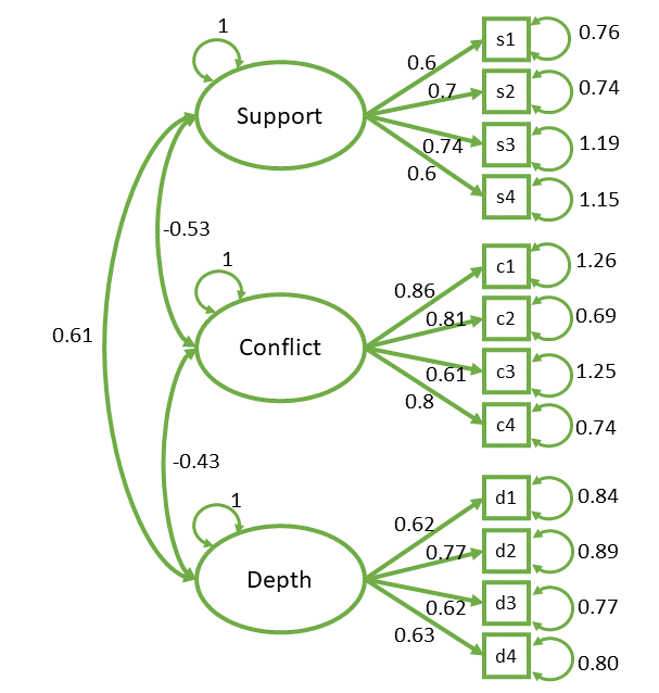
example: QRI
qri <- read.csv("https://uoepsy.github.io/data/qri.csv")
head(qri)
s2 d4 c3 c4 d1 c2 s1 s4 d2 c1 s3 d3
1 4 4 5 5 5 4 3 3 2 3 5 5
2 3 5 4 4 2 4 4 5 2 4 4 4
3 4 5 4 5 4 2 5 3 6 2 4 5
4 3 6 4 3 5 3 3 4 4 2 5 5
5 6 7 1 2 4 2 7 7 4 1 7 5
6 3 5 5 4 4 3 5 4 3 3 5 5mymod <- "
support =~ s1 + s2 + s3 + s4
conflict =~ c1 + c2 + c3 + c4
depth =~ d1 + d2 + d3 + d4
support ~~ conflict
support ~~ depth
conflict ~~ depth
"
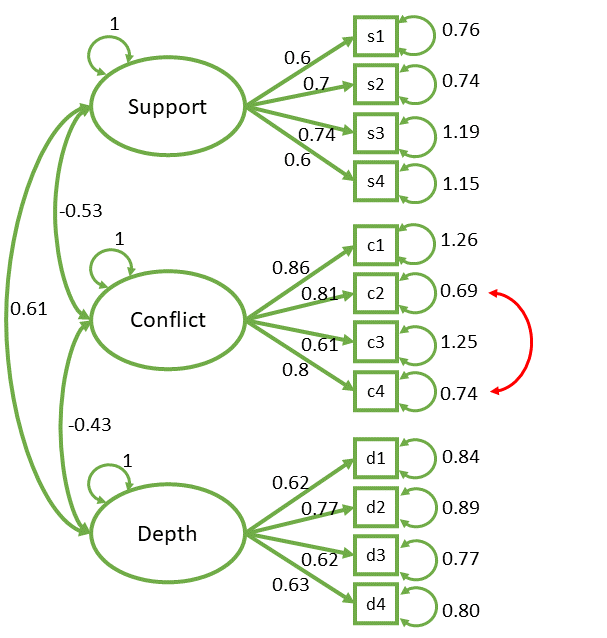
mymod.est <- cfa(mymod, data = qri, std.lv = TRUE)example: QRI
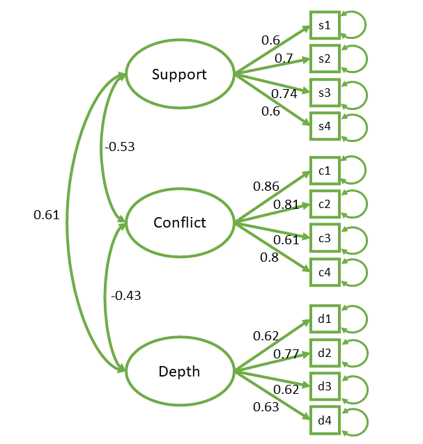
summary(mymod.est)lavaan 0.6-19 ended normally after 19 iterations
Estimator ML
Optimization method NLMINB
Number of model parameters 27
Number of observations 374
Model Test User Model:
Test statistic 81.100
Degrees of freedom 51
P-value (Chi-square) 0.005
Parameter Estimates:
Standard errors Standard
Information Expected
Information saturated (h1) model Structured
Latent Variables:
Estimate Std.Err z-value P(>|z|)
support =~
s1 0.601 0.062 9.765 0.000
s2 0.707 0.064 11.010 0.000
s3 0.642 0.074 8.676 0.000
s4 0.608 0.072 8.407 0.000
conflict =~
c1 0.860 0.077 11.102 0.000
c2 0.810 0.063 12.909 0.000
c3 0.614 0.072 8.532 0.000
c4 0.808 0.064 12.673 0.000
depth =~
d1 0.617 0.063 9.759 0.000
d2 0.770 0.069 11.175 0.000
d3 0.621 0.061 10.119 0.000
d4 0.634 0.062 10.143 0.000
Covariances:
Estimate Std.Err z-value P(>|z|)
support ~~
conflict -0.530 0.063 -8.473 0.000
depth 0.613 0.062 9.956 0.000
conflict ~~
depth -0.425 0.065 -6.551 0.000
Variances:
Estimate Std.Err z-value P(>|z|)
.s1 0.763 0.070 10.860 0.000
.s2 0.738 0.077 9.626 0.000
.s3 1.188 0.102 11.625 0.000
.s4 1.151 0.098 11.781 0.000
.c1 1.259 0.116 10.893 0.000
.c2 0.692 0.076 9.128 0.000
.c3 1.251 0.102 12.276 0.000
.c4 0.735 0.078 9.409 0.000
.d1 0.839 0.075 11.146 0.000
.d2 0.885 0.089 9.923 0.000
.d3 0.771 0.071 10.880 0.000
.d4 0.797 0.073 10.861 0.000
support 1.000
conflict 1.000
depth 1.000 example: QRI
summary(mymod.est)lavaan 0.6-19 ended normally after 19 iterations
Estimator ML
Optimization method NLMINB
Number of model parameters 27
Number of observations 374
Model Test User Model:
Test statistic 81.100
Degrees of freedom 51
P-value (Chi-square) 0.005
Parameter Estimates:
Standard errors Standard
Information Expected
Information saturated (h1) model Structured
Latent Variables:
Estimate Std.Err z-value P(>|z|)
support =~
s1 0.601 0.062 9.765 0.000
s2 0.707 0.064 11.010 0.000
s3 0.642 0.074 8.676 0.000
s4 0.608 0.072 8.407 0.000
conflict =~
c1 0.860 0.077 11.102 0.000
c2 0.810 0.063 12.909 0.000
c3 0.614 0.072 8.532 0.000
c4 0.808 0.064 12.673 0.000
depth =~
d1 0.617 0.063 9.759 0.000
d2 0.770 0.069 11.175 0.000
d3 0.621 0.061 10.119 0.000
d4 0.634 0.062 10.143 0.000
Covariances:
Estimate Std.Err z-value P(>|z|)
support ~~
conflict -0.530 0.063 -8.473 0.000
depth 0.613 0.062 9.956 0.000
conflict ~~
depth -0.425 0.065 -6.551 0.000
Variances:
Estimate Std.Err z-value P(>|z|)
.s1 0.763 0.070 10.860 0.000
.s2 0.738 0.077 9.626 0.000
.s3 1.188 0.102 11.625 0.000
.s4 1.151 0.098 11.781 0.000
.c1 1.259 0.116 10.893 0.000
.c2 0.692 0.076 9.128 0.000
.c3 1.251 0.102 12.276 0.000
.c4 0.735 0.078 9.409 0.000
.d1 0.839 0.075 11.146 0.000
.d2 0.885 0.089 9.923 0.000
.d3 0.771 0.071 10.880 0.000
.d4 0.797 0.073 10.861 0.000
support 1.000
conflict 1.000
depth 1.000 what are the model parameters?
the estimated paths on the diagram!
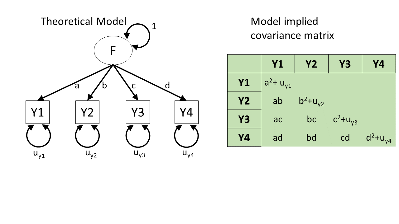
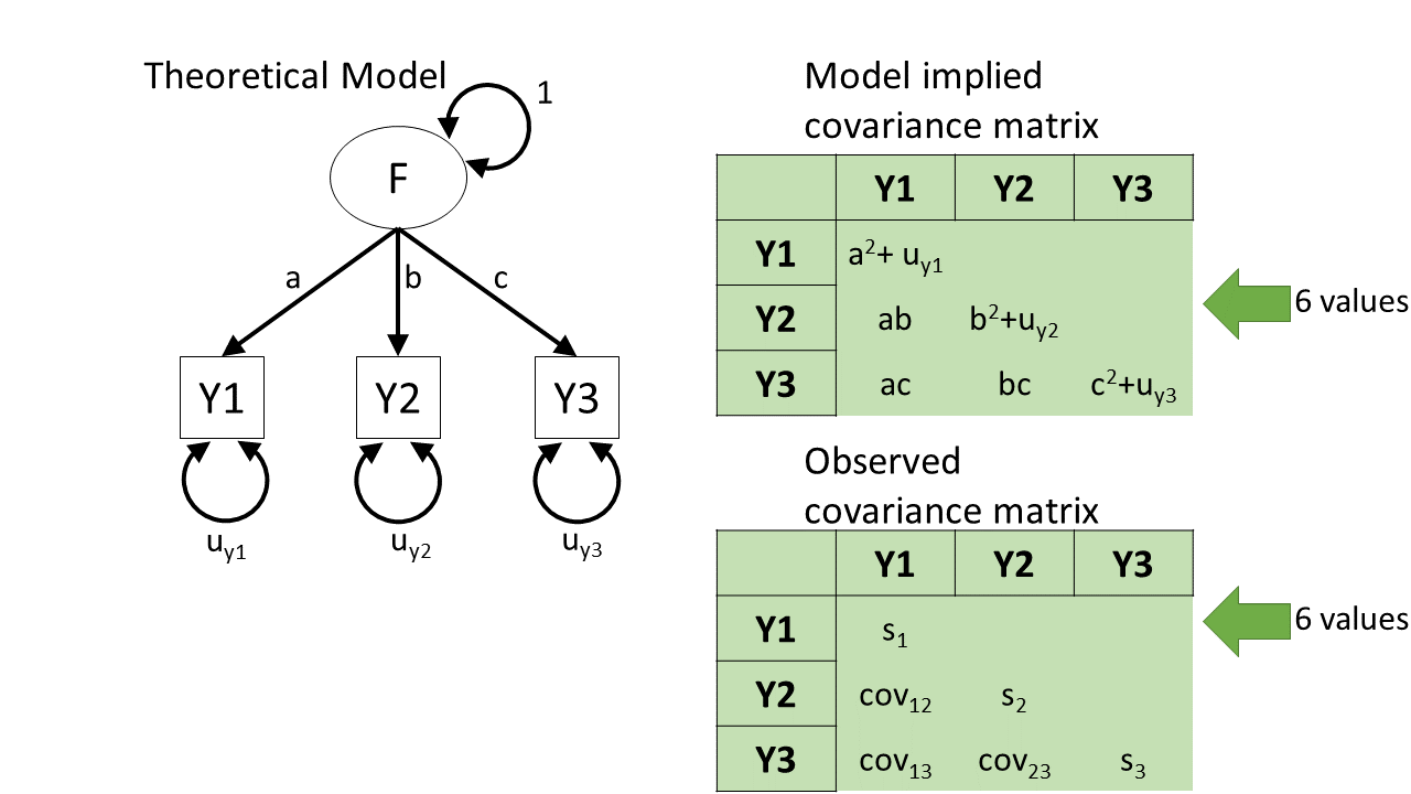
how does a diagram imply a covariance?
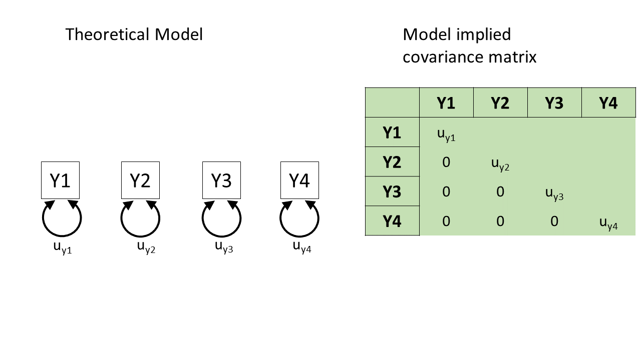
how does a diagram imply a covariance? (2)
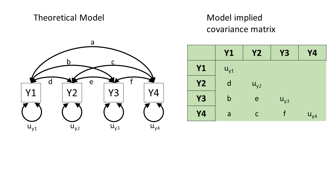
how does a diagram imply a covariance? (3)
identifiability
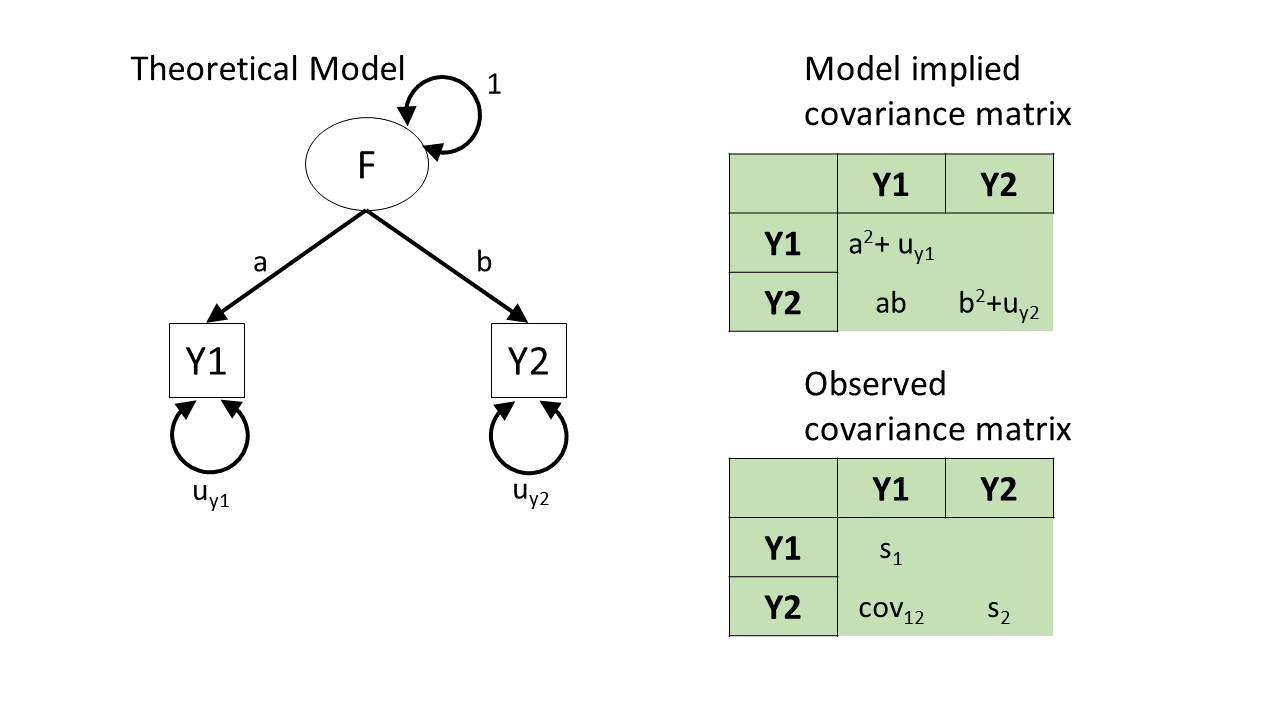
identifiability (2)
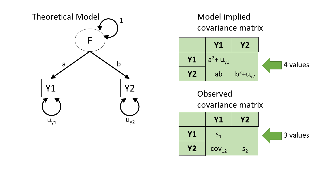
identifiability (3)
example: QRI
how many “knowns”?
cov(qri) |>
  round(2)
s2 d4 c3 c4 d1 c2 s1 s4 d2 c1 s3 d3
s2 1.24 0.32 -0.26 -0.24 0.22 -0.21 0.46 0.39 0.39 -0.46 0.44 0.31
d4 0.32 1.20 -0.19 -0.10 0.39 -0.20 0.20 0.29 0.47 -0.40 0.24 0.41
c3 -0.26 -0.19 1.63 0.41 -0.24 0.43 -0.31 -0.32 -0.34 0.68 -0.24 -0.29
c4 -0.24 -0.10 0.41 1.39 -0.15 0.78 -0.24 -0.24 -0.16 0.62 -0.29 -0.14
d1 0.22 0.39 -0.24 -0.15 1.22 -0.22 0.19 0.16 0.51 -0.42 0.24 0.38
c2 -0.21 -0.20 0.43 0.78 -0.22 1.35 -0.18 -0.18 -0.17 0.62 -0.26 -0.20
s1 0.46 0.20 -0.31 -0.24 0.19 -0.18 1.13 0.36 0.28 -0.38 0.37 0.20
s4 0.39 0.29 -0.32 -0.24 0.16 -0.18 0.36 1.53 0.29 -0.45 0.45 0.24
d2 0.39 0.47 -0.34 -0.16 0.51 -0.17 0.28 0.29 1.48 -0.37 0.32 0.46
c1 -0.46 -0.40 0.68 0.62 -0.42 0.62 -0.38 -0.45 -0.37 2.00 -0.30 -0.32
s3 0.44 0.24 -0.24 -0.29 0.24 -0.26 0.37 0.45 0.32 -0.30 1.61 0.23
d3 0.31 0.41 -0.29 -0.14 0.38 -0.20 0.20 0.24 0.46 -0.32 0.23 1.16how many “unknowns”?
modification indices
| var | wording |
|---|---|
| s1 | To what extent could you turn to this person for advice about problems? |
| s2 | To what extent could you count on this person for help with a problem? |
| s3 | To what extent can you really count on this person to distract you from your worries when you feel under stress? |
| s4 | To what extent can you count on this person to listen to you when you are very angry at someone else? |
| c1 | How often do you have to work hard to avoid conflict with this person? |
| c2 | How much do you argue with this person? |
| c3 | How much would you like this person to change? |
| c4 | How often does this person make you feel angry? |
| d1 | How positive a role does this person play in your life? |
| d2 | How significant is this relationship in your life? |
| d3 | How close will your relationship be with this person in 10 years? |
| d4 | How much would you miss this person if the two of you could not see or talk with each other for a month? |
beyond this point
stuff beyond here definitely won’t be in the exam or in the quiz.

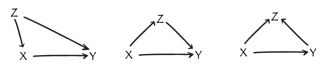
graphical models
there’s a formal logic to diagrams (“do-calculus”).
mainly for back-of-envelope thinking
essentially a way of helping to figure out how to get at an unbiased estimate of the thing we are interested in.
helps with thinking about any part of a study that is observed not manipulated/randomly allocated
I surreptitiously introduced you to this way of thinking in back in Week 1!
error error everywhere

SEM
There’s error everywhere!
Models can have structural parts and measurement parts. It all gets estimated at once!
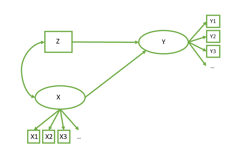
# measurement model
Y =~ y1 + y2 + y3 + ...
X =~ x1 + x2 + x3 + ...
# regressions
Y ~ X + Z
# covariances
X ~~ Z
common uses of SEM
“Nomological Net”
Do things correlate with other things we expect them to correlate with?
Good for assessing if our measure is measuring the thing we want it to measure!
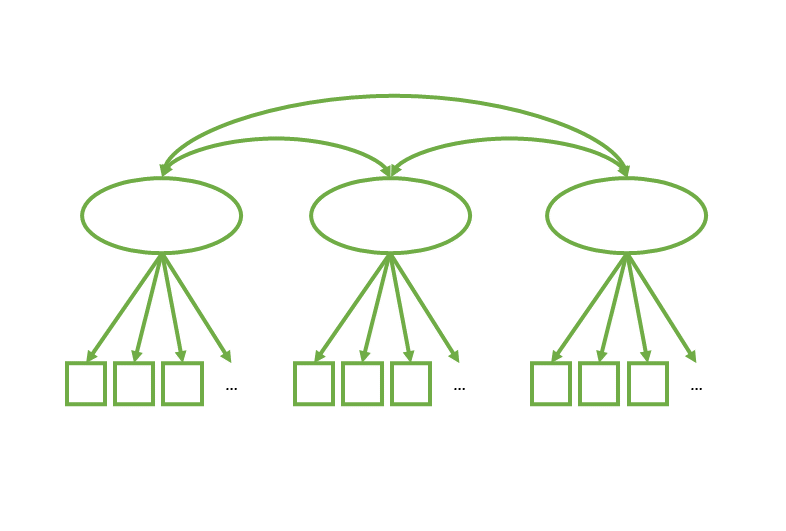
# measurement model
F1 =~ y1 + y2 + y3 + ...
F2 =~ x1 + x2 + x3 + ...
F3 =~ w1 + w2 + w3 + ...
# latent variable covariances
F1 ~~ F2
F1 ~~ F3
F2 ~~ F3
common uses of SEM
Measurement Invariance
Do factor loadings differ between groups/timepoints/contexts?

F1 =~ y1 + y2 + y3 + ...m1 <- cfa(model, data, group = "mygroups")
m2 <- cfa(model, data, group = "mygroups",
group.equal = "loadings")
semTools::compareFit(m1,m2)common uses of SEM
Mediation
How much of X -> Y is because of X -> M and M -> Y?
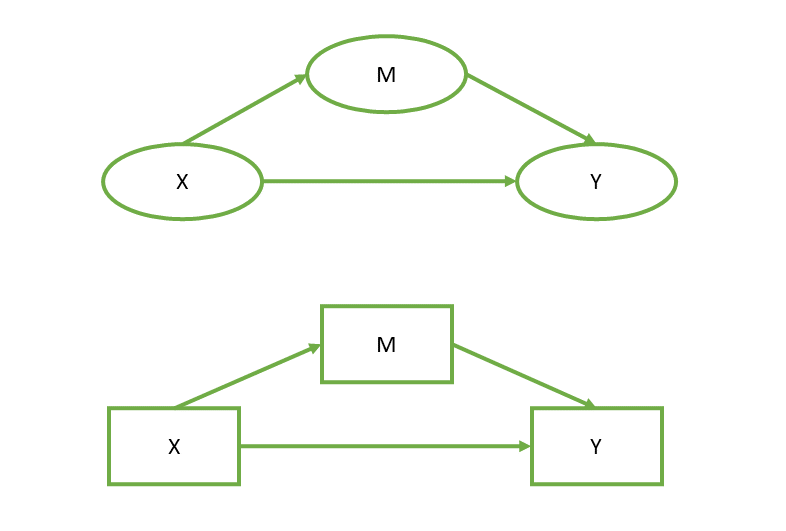
Y ~ a*M + c*X
M ~ b*X
indirect := a*b
direct := c
sem(model, data)⚠ mediation is almost always incredibly problematic. Many people dismiss it altogether as essentially useless because confounding is everywhere.
cross-sectional observational mediation = “three correlations in a trenchcoat”1
common uses of SEM
Latent Growth Curves
The same as lmer(Y ~ TimePoint + (1 + TimePoint | Person))
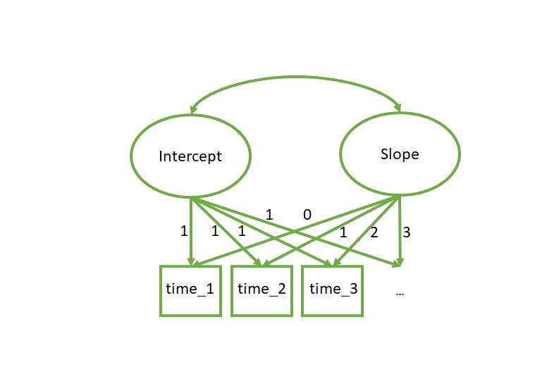
int =~ 1*Time1 + 1*Time2 + 1*Time3 + ...
slope =~ 0*Time1 + 1*Time2 + 2*Time3 + ...
int ~~ slope
growth(model, data)