
Assumptions, Diagnostics, and Centering
Data Analysis for Psychology in R 3
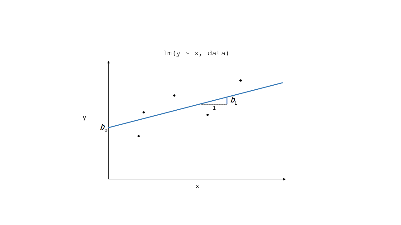
Resids
Resids (2)
Resids (3)
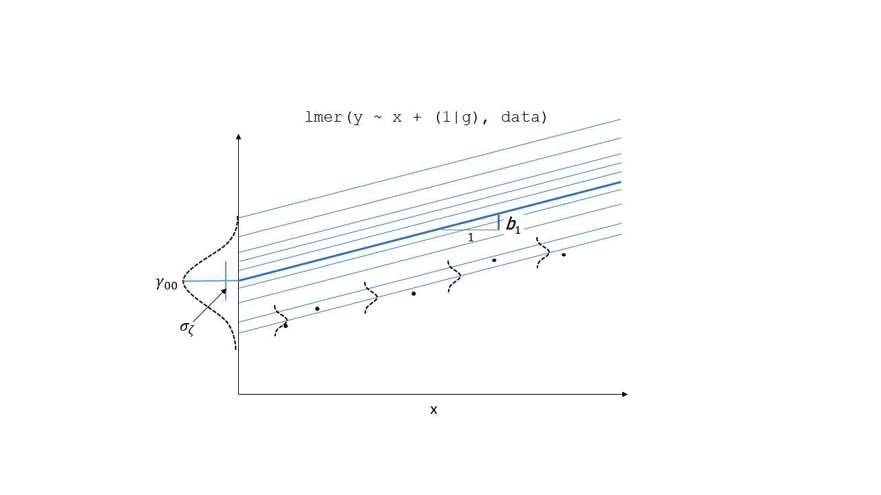
Random effects as level 2 residuals
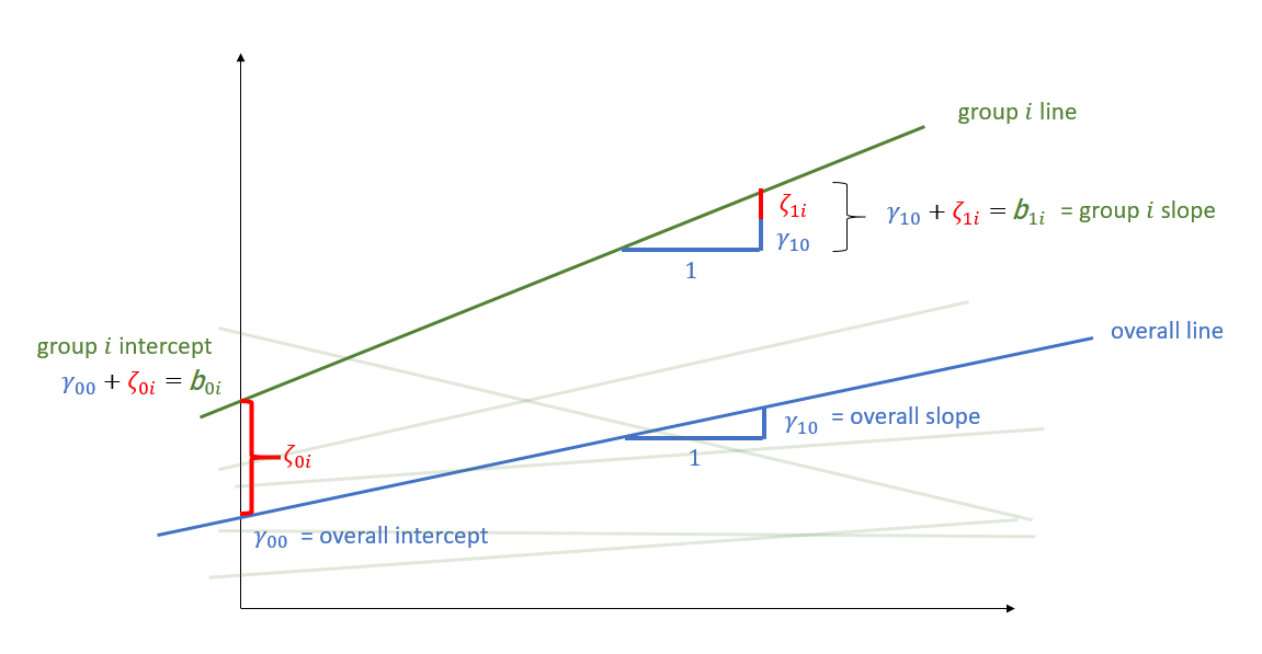
Random effects as level 2 residuals
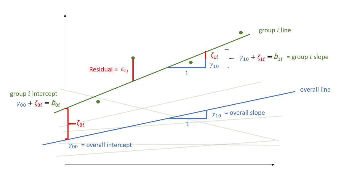
Random effects as level 2 residuals
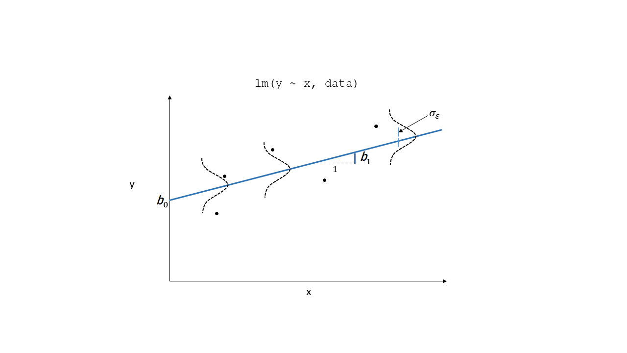
\(\varepsilon\)
resid(model)
zero mean, constant variance

\(\color{orange}{\zeta}\)
ranef(model)
zero mean, constant variance
$cluster
Assumption Plots: Residuals vs Fitted
plot(model, type=c("p","smooth"))
Assumption Plots: qqplots
qqnorm(resid(model))
qqline(resid(model))
Assumption Plots: Scale-Location
plot(model,
     form = sqrt(abs(resid(.))) ~ fitted(.),
     type = c("p","smooth"))
Assumption Plots: Scale-Location
plot(model,
     form = sqrt(abs(resid(.))) ~ fitted(.) | cluster,
     type = c("p"))
Assumption Plots: Ranefs
base
qqnorm(ranef(model)$cluster[,1])
qqline(ranef(model)$cluster[,1])
qqnorm(ranef(model)$cluster[,2])
qqline(ranef(model)$cluster[,2])
ggplot
rans <- as.data.frame(ranef(model)$cluster)

ggplot(rans, aes(sample = `(Intercept)`)) +
  stat_qq() + stat_qq_line() +
  labs(title="random intercept")

ggplot(rans, aes(sample = x1)) +
  stat_qq() + stat_qq_line()
  labs(title="random slope")
“posterior” predictions
performance::check_predictions(model)
!?!?!?!

Assumptions are not either “violated” or “not violated”.
Assumptions are the things we assume when ‘using’ a model.
- the question is whether we (given our plots etc) are happy to assume these things
Same old study
In a study examining how cognition changes over time, a sample of 20 participants took the Addenbrooke’s Cognitive Examination (ACE) every 2 years from age 60 to age 78.
Each participant has 10 datapoints. Participants are clusters.
d3 <- read_csv("https://uoepsy.github.io/data/lmm_mindfuldecline.csv")
head(d3)
# A tibble: 6 × 7
sitename ppt condition visit age ACE imp
<chr> <chr> <chr> <dbl> <dbl> <dbl> <chr>
1 Sncbk PPT_1 control 1 60 84.5 unimp
2 Sncbk PPT_1 control 2 62 85.6 imp
3 Sncbk PPT_1 control 3 64 84.5 imp
4 Sncbk PPT_1 control 4 66 83.1 imp
5 Sncbk PPT_1 control 5 68 82.3 imp
6 Sncbk PPT_1 control 6 70 83.3 imp 
Model mis-specification
mymodel <- lmer(ACE ~ visit * condition + (1 | ppt), data = d3)
performance::check_model(mymodel)
Model mis-specification
mymodel <- lmer(ACE ~ visit * condition +
                  (1 | ppt), data = d3)
mymodel <- lmer(ACE ~ visit * condition +
                  (1 + visit | ppt), data = d3)
Modelling a different form of relation
Transformations
- Transforming your outcome variable may result in a model with better looking assumption plots
lmer(y ~ x1 + c +
       (1 | cluster), df)
lmer(forecast::BoxCox(y,lambda="auto") ~ x1 + c +
       (1 | cluster), df)
Case Bootstrap
NOT IMPLEMENTED FOR CROSSED STRUCTURES
mymodel <- lmer(ACE ~ visit * condition + (1 + visit | ppt), data = d3)

library(lmeresampler)
# resample only the people, not their observations:
mymodelBScase <- bootstrap(mymodel, .f = fixef,
                           type = "case", B = 1000,
resample = c(TRUE, FALSE))confint(mymodelBScase, type = "perc")# A tibble: 4 × 6
term estimate lower upper type level
<chr> <dbl> <dbl> <dbl> <chr> <dbl>
1 (Intercept) 85.7 85.5 86.0 perc 0.95
2 visit -0.532 -0.666 -0.390 perc 0.95
3 conditionmindfulness -0.298 -0.650 0.0736 perc 0.95
4 visit:conditionmindfulness 0.346 0.151 0.555 perc 0.95For a discussion of different bootstrap methods for multilevel models, see Leeden R.., Meijer E., Busing F.M. (2008) Resampling Multilevel Models. In: Leeuw J.., Meijer E. (eds) Handbook of Multilevel Analysis. Springer, New York, NY. DOI: 10.1007/978-0-387-73186-5_11
plot(mymodelBScase, "visit*conditionmindfulness")
Influence
Just like standard lm(), observations can have unduly high influence on our model through a combination of high leverage and outlyingness.

Level 1 influential points
mymodel <- lmer(ACE ~ visit * condition +
                  (1 + visit | ppt), data = d3)


library(HLMdiag)
infl1 <- hlm_influence(mymodel, level = 1)
infl2 <- hlm_influence(mymodel, level = "ppt")dotplot_diag(infl1$cooksd, cutoff = "internal")
Level 2 influential clusters
mymodel <- lmer(ACE ~ visit * condition +
                  (1 + visit | ppt), data = d3)


library(HLMdiag)
infl1 <- hlm_influence(mymodel, level = 1)
infl2 <- hlm_influence(mymodel, level = "ppt")dotplot_diag(infl2$cooksd, cutoff = "internal", index=infl2$ppt)dotplot_diag(infl2$cooksd, cutoff = 0.201, index=infl2$ppt)
Centering
Suppose we have a variable for which the mean is 100.

We can re-center this so that 100 (the mean) becomes zero:

Centering
Suppose we have a variable for which the mean is 100.

We can re-center this so that any value becomes zero:

Scaling
Suppose we have a variable for which the mean is 100. The standard deviation is 15

We can scale this so that a change in 1 is equivalent to a change in 1 standard deviation:

Centering predictors in LM
m1 <- lm(y~x,data=df)
m2 <- lm(y~scale(x, center=T,scale=F),data=df)
m3 <- lm(y~scale(x, center=T,scale=T),data=df)
m4 <- lm(y~I(x-5), data=df)anova(m1,m2,m3,m4)Analysis of Variance Table
Model 1: y ~ x
Model 2: y ~ scale(x, center = T, scale = F)
Model 3: y ~ scale(x, center = T, scale = T)
Model 4: y ~ I(x - 5)
Res.Df RSS Df Sum of Sq F Pr(>F)
1 198 177
2 198 177 0 -2.84e-14
3 198 177 0 0.00e+00
4 198 177 0 0.00e+00 
Big Fish Little Fish

Big Fish Little Fish

data available at https://uoepsy.github.io/data/bflp.csv
Things are different with multi-level data

Multiple means
Grand mean

Group means

Group-mean centering
Group-mean centering
\(x_{ij} - \bar{x}_i\)

\(\bar{x}_i\)

Disaggregating within & between

Within-between model
\[
\begin{align}
y_{ij} &= b_{0i} + b_{1}(\bar{x}_i) + b_2(x_{ij} - \bar{x}_i)+ \varepsilon_{ij} \\
b_{0i} &= \gamma_{00} + \zeta_{0i} \\
... \\
\end{align}
\]
bflp <-
  bflp |> group_by(pond) |>
    mutate(
      fw_between_pond = mean(fish_weight),
      fw_within_pond = fish_weight - mean(fish_weight)
    ) |> ungroup()

mod_wb <- lmer(self_esteem ~ fw_between_pond + fw_within_pond +
              (1 | pond), data=bflp)
fixef(mod_wb)
(Intercept) fw_between_pond fw_within_pond
4.7680 -0.0559 0.0407 A more realistic example
A research study investigates how anxiety is associated with drinking habits. Data was collected from 50 participants. Researchers administered the generalised anxiety disorder (GAD-7) questionnaire to measure levels of anxiety over the past week, and collected information on the units of alcohol participants had consumed within the week. Each participant was observed on 10 different occasions.

data available at https://uoepsy.github.io/data/lmm_alcgad.csv
A more realistic example
The Within Question
Is being more anxious (than you usually are) associated with higher consumption of alcohol?

A more realistic example
The Between Question
Is being generally more anxious (relative to others) associated with higher consumption of alcohol?

Within & Between effects


Within & Between effects


This week
Tasks
 Complete readings
 Attend your lab and work together on the exercises
 Complete the weekly quiz
Support
 Piazza forum!
 Office hours (see Learn page for details)