Multilevel Models

Data Analysis for Psychology in R 3

Josiah King

Psychology, PPLS

University of Edinburgh

Overview

multilevel modelling working with group structured data	regression refresher
	the multilevel model
	more complex groupings
	centering, assumptions, and diagnostics
	recap
factor analysis working with multi-item measures	measurement and dimensionality
	exploring underlying constructs (EFA)
	testing theoretical models (CFA)
	reliability and validity
	recap & exam prep

This week

• introduction to the multilevel/mixed effects model
  • how to think about it (model structure)
  • how to fit it (in R)

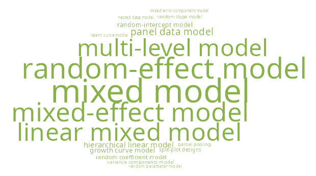
Terminology

(size weighted by hits on google scholar)

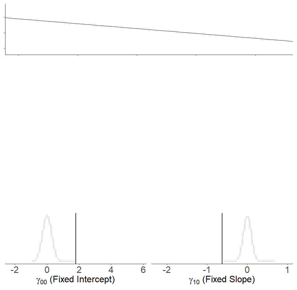
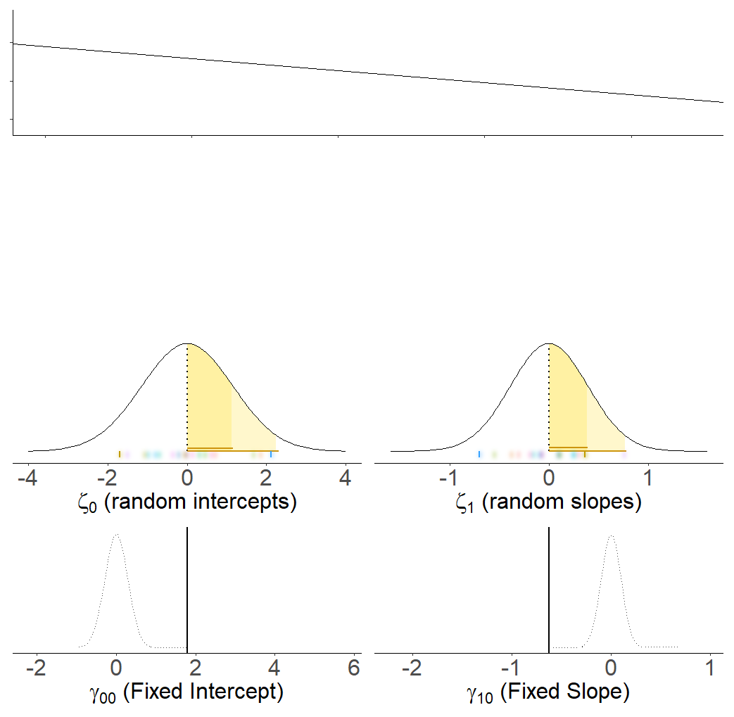
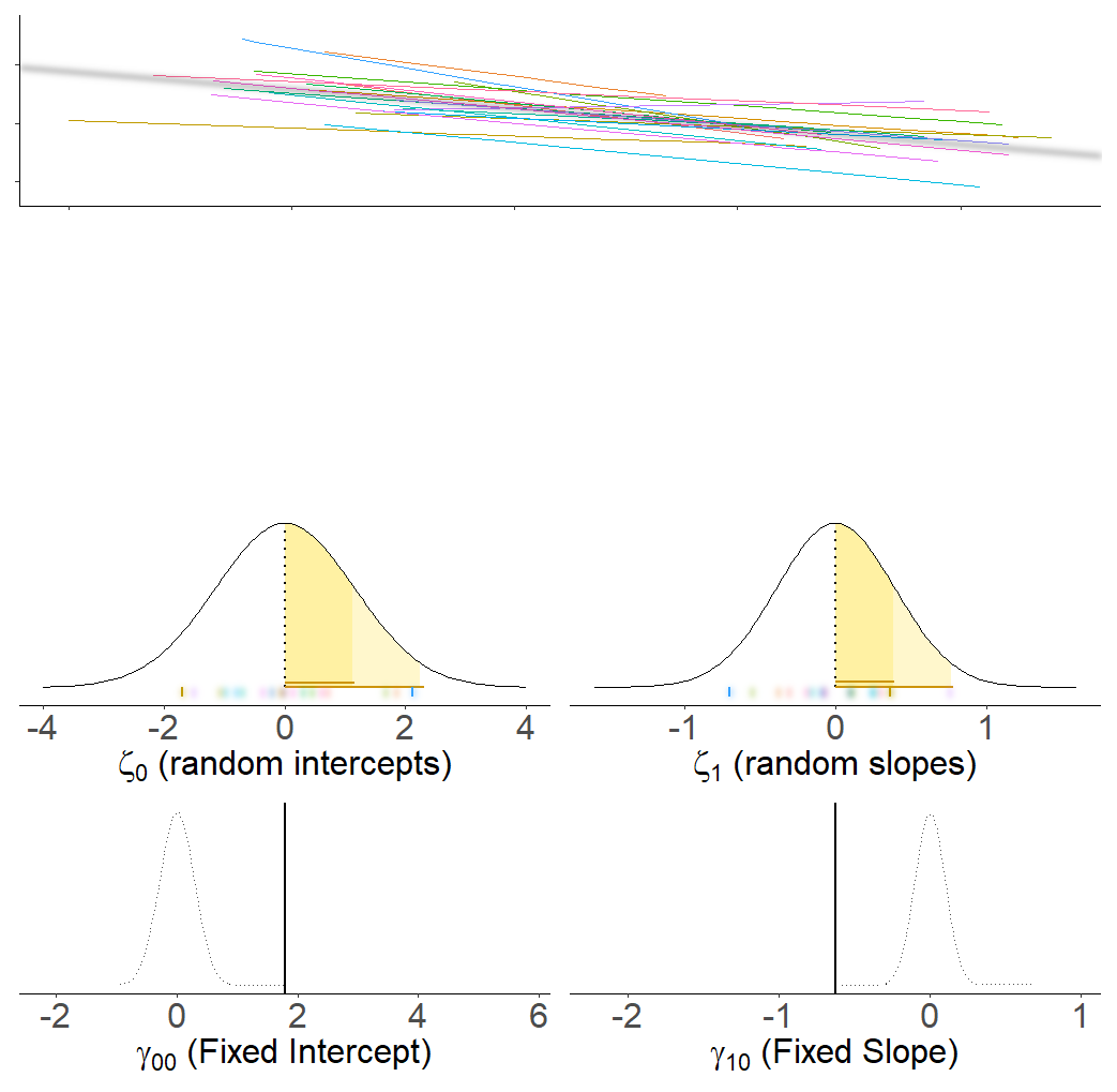
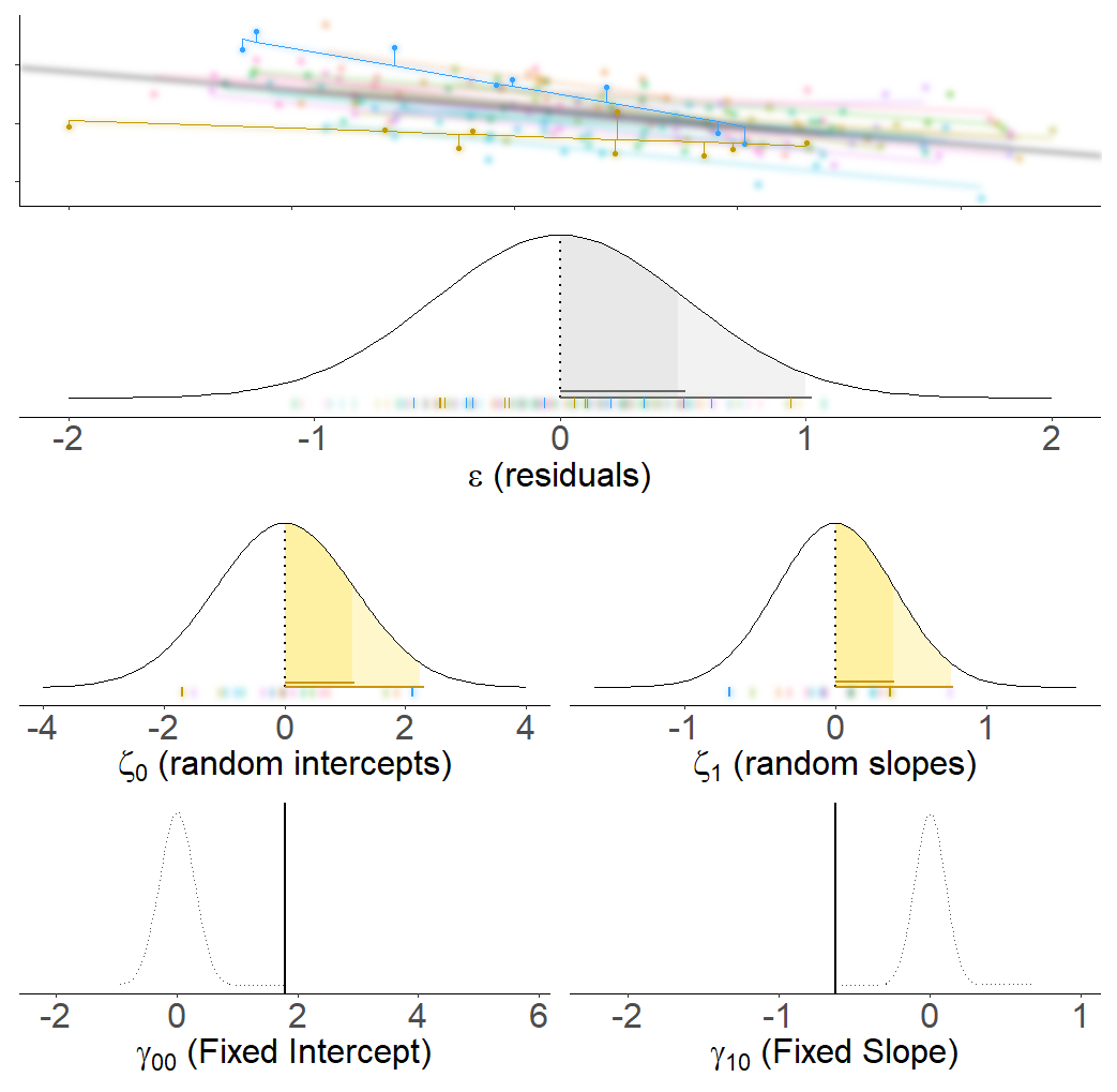
Building up the idea - in pictures

back to our example

Are older people more satisfied with life? 112 people from 12 different dwellings (cities/towns) in Scotland. Information on their ages and some measure of life satisfaction.

d3 <- read_csv("https://uoepsy.github.io/data/lmm_lifesatscot.csv") 
head(d3)

# A tibble: 6 × 4
    age lifesat dwelling size 
  <dbl>   <dbl> <chr>    <chr>
1    40      31 Aberdeen >100k
2    45      56 Glasgow  >100k
3    40      51 Glasgow  >100k
4    40      55 Dundee   >100k
5    40      41 Dundee   >100k
6    55      69 Perth    <100k

estimate the differences

the fixed effects approach:

mod <- lm(lifesat ~ 1 + dwelling + age, data = d3)
summary(mod)

Call:
lm(formula = lifesat ~ 1 + dwelling + age, data = d3)

Residuals:
    Min      1Q  Median      3Q     Max 
-17.144  -5.463  -0.772   6.074  20.432 

Coefficients:
                     Estimate Std. Error t value Pr(>|t|)    
(Intercept)           15.3330     4.1493    3.70  0.00036 ***
dwellingDumfries       8.0741     3.8483    2.10  0.03844 *  
dwellingDundee        15.9882     3.8236    4.18  6.3e-05 ***
dwellingDunfermline   26.2600     3.8910    6.75  1.0e-09 ***
dwellingEdinburgh     12.6929     3.8195    3.32  0.00125 ** 
dwellingFort William   1.3577     3.8999    0.35  0.72849    
dwellingGlasgow       18.2906     3.8213    4.79  5.9e-06 ***
dwellingInverness      5.0718     3.8542    1.32  0.19124    
dwellingKirkcaldy    -22.5918     6.8344   -3.31  0.00132 ** 
dwellingPaisley        1.6647     3.8748    0.43  0.66840    
dwellingPerth         14.1953     3.8182    3.72  0.00033 ***
dwellingStirling      17.6765     3.8429    4.60  1.3e-05 ***
age                    0.6047     0.0888    6.81  7.6e-10 ***
---
Signif. codes:  0 '***' 0.001 '**' 0.01 '*' 0.05 '.' 0.1 ' ' 1

Residual standard error: 8.54 on 99 degrees of freedom
Multiple R-squared:  0.622, Adjusted R-squared:  0.577 
F-statistic: 13.6 on 12 and 99 DF,  p-value: 3.77e-16

estimate the differences

the fixed effects approach:

mod <- lm(lifesat ~ 1 + dwelling + age, data = d3)
summary(mod)

Call:
lm(formula = lifesat ~ 1 + dwelling + age, data = d3)

Residuals:
    Min      1Q  Median      3Q     Max 
-17.144  -5.463  -0.772   6.074  20.432 

Coefficients:
                     Estimate Std. Error t value Pr(>|t|)    
(Intercept)           15.3330     4.1493    3.70  0.00036 ***
dwellingDumfries       8.0741     3.8483    2.10  0.03844 *  
dwellingDundee        15.9882     3.8236    4.18  6.3e-05 ***
dwellingDunfermline   26.2600     3.8910    6.75  1.0e-09 ***
dwellingEdinburgh     12.6929     3.8195    3.32  0.00125 ** 
dwellingFort William   1.3577     3.8999    0.35  0.72849    
dwellingGlasgow       18.2906     3.8213    4.79  5.9e-06 ***
dwellingInverness      5.0718     3.8542    1.32  0.19124    
dwellingKirkcaldy    -22.5918     6.8344   -3.31  0.00132 ** 
dwellingPaisley        1.6647     3.8748    0.43  0.66840    
dwellingPerth         14.1953     3.8182    3.72  0.00033 ***
dwellingStirling      17.6765     3.8429    4.60  1.3e-05 ***
age                    0.6047     0.0888    6.81  7.6e-10 ***
---
Signif. codes:  0 '***' 0.001 '**' 0.01 '*' 0.05 '.' 0.1 ' ' 1

Residual standard error: 8.54 on 99 degrees of freedom
Multiple R-squared:  0.622, Adjusted R-squared:  0.577 
F-statistic: 13.6 on 12 and 99 DF,  p-value: 3.77e-16

estimate the differences

the fixed effects approach:

mod <- lm(lifesat ~ 1 + dwelling + age, data = d3)
summary(mod)

Call:
lm(formula = lifesat ~ 1 + dwelling + age, data = d3)

Residuals:
    Min      1Q  Median      3Q     Max 
-17.144  -5.463  -0.772   6.074  20.432 

Coefficients:
                     Estimate Std. Error t value Pr(>|t|)    
(Intercept)           15.3330     4.1493    3.70  0.00036 ***
dwellingDumfries       8.0741     3.8483    2.10  0.03844 *  
dwellingDundee        15.9882     3.8236    4.18  6.3e-05 ***
dwellingDunfermline   26.2600     3.8910    6.75  1.0e-09 ***
dwellingEdinburgh     12.6929     3.8195    3.32  0.00125 ** 
dwellingFort William   1.3577     3.8999    0.35  0.72849    
dwellingGlasgow       18.2906     3.8213    4.79  5.9e-06 ***
dwellingInverness      5.0718     3.8542    1.32  0.19124    
dwellingKirkcaldy    -22.5918     6.8344   -3.31  0.00132 ** 
dwellingPaisley        1.6647     3.8748    0.43  0.66840    
dwellingPerth         14.1953     3.8182    3.72  0.00033 ***
dwellingStirling      17.6765     3.8429    4.60  1.3e-05 ***
age                    0.6047     0.0888    6.81  7.6e-10 ***
---
Signif. codes:  0 '***' 0.001 '**' 0.01 '*' 0.05 '.' 0.1 ' ' 1

Residual standard error: 8.54 on 99 degrees of freedom
Multiple R-squared:  0.622, Adjusted R-squared:  0.577 
F-statistic: 13.6 on 12 and 99 DF,  p-value: 3.77e-16

estimate the differences

the fixed effects approach:

mod <- lm(lifesat ~ 1 + dwelling + age, data = d3)
summary(mod)

Call:
lm(formula = lifesat ~ 1 + dwelling + age, data = d3)

Residuals:
    Min      1Q  Median      3Q     Max 
-17.144  -5.463  -0.772   6.074  20.432 

Coefficients:
                     Estimate Std. Error t value Pr(>|t|)    
(Intercept)           15.3330     4.1493    3.70  0.00036 ***
dwellingDumfries       8.0741     3.8483    2.10  0.03844 *  
dwellingDundee        15.9882     3.8236    4.18  6.3e-05 ***
dwellingDunfermline   26.2600     3.8910    6.75  1.0e-09 ***
dwellingEdinburgh     12.6929     3.8195    3.32  0.00125 ** 
dwellingFort William   1.3577     3.8999    0.35  0.72849    
dwellingGlasgow       18.2906     3.8213    4.79  5.9e-06 ***
dwellingInverness      5.0718     3.8542    1.32  0.19124    
dwellingKirkcaldy    -22.5918     6.8344   -3.31  0.00132 ** 
dwellingPaisley        1.6647     3.8748    0.43  0.66840    
dwellingPerth         14.1953     3.8182    3.72  0.00033 ***
dwellingStirling      17.6765     3.8429    4.60  1.3e-05 ***
age                    0.6047     0.0888    6.81  7.6e-10 ***
---
Signif. codes:  0 '***' 0.001 '**' 0.01 '*' 0.05 '.' 0.1 ' ' 1

Residual standard error: 8.54 on 99 degrees of freedom
Multiple R-squared:  0.622, Adjusted R-squared:  0.577 
F-statistic: 13.6 on 12 and 99 DF,  p-value: 3.77e-16

deviations from an average

Group deviations from an overall average

deviations from an average

Group deviations from an overall average

deviations from an average

Group deviations from an overall average

the multilevel model: a model of models?

models group-level variability, rather than estimating group differences.

think “a distribution of possible lines”

Checkpoint!

Building up the idea - in equations

single level regression

\[ \begin{align} & \text{for observation }j \\ \quad \\ & \text{ } \\ & \color{red}{y_j} = \color{blue}{b_0 \cdot{} 1 \; + \; b_1 \cdot{} x_{j} } + \varepsilon_j \\ \end{align} \]

for observation \(j\),

their value of \(\color{red}{y}\) =
  some number (\(\color{blue}{b_0}\)) +
  some amount (\(\color{blue}{b_1}\)) times their value of \(x\) +
  their residual \(\varepsilon_j\)

multi-level regression

\[ \begin{align} & \text{for observation }j\text{ in group }i \\ \quad \\ & \text{Level 1:} \\ & \color{red}{y_{ij}} = \color{blue}{b_{0i} \cdot 1 + b_{1} \cdot x_{ij}} + \varepsilon_{ij} \\ \end{align} \]

for observation \(j\) from group \(i\),

their value of \(\color{red}{y}\) =
  some number for group \(i\) (\(\color{blue}{b_{0i}}\)) +
  some amount (\(\color{blue}{b_1}\)) times their value of \(x\) +
  their residual \(\varepsilon_{ij}\)

multi-level regression

\[ \begin{align} & \text{for observation }j\text{ in group }i \\ \quad \\ & \text{Level 1:} \\ & \color{red}{y_{ij}} = \color{blue}{b_{0i} \cdot 1 + b_{1} \cdot x_{ij}} + \varepsilon_{ij} \\ & \quad \\ & \text{Level 2:} \\ & \color{blue}{b_{0i}} = \gamma_{00} + \color{orange}{\zeta_{0i}} \\ \quad \\ \end{align} \]

for observation \(j\) from group \(i\),

their value of \(\color{red}{y}\) =
  some number for group \(i\) (\(\color{blue}{b_{0i}}\)) +
  some amount (\(\color{blue}{b_1}\)) times their value of \(x\) +
  their residual \(\varepsilon_{ij}\)

group \(i\)’s intercept (\(\color{blue}{b_{0i}}\)) =
  the intercept for the average of the population of groups (\(\gamma_{00}\)) +
  the deviation of group \(i\) (\(\color{orange}{\zeta_{0i}}\)) from \(\gamma_{00}\)

multi-level regression

\[ \begin{align} & \text{for observation }j\text{ in group }i \\ \quad \\ & \text{Level 1:} \\ & \color{red}{y_{ij}} = \color{blue}{b_{0i} \cdot 1 + b_{1} \cdot x_{ij}} + \varepsilon_{ij} \\ & \quad \\ & \text{Level 2:} \\ & \color{blue}{b_{0i}} = \gamma_{00} + \color{orange}{\zeta_{0i}} \\ \quad \\ & \color{orange}{\zeta_{0i}} \sim N(0, \color{orange}{\sigma^2_0}) \\ & \varepsilon_{ij} \sim N(0, \sigma^2_\varepsilon) \\ \end{align} \]

for observation \(j\) from group \(i\),

their value of \(\color{red}{y}\) =
  some number for group \(i\) (\(\color{blue}{b_{0i}}\)) +
  some amount (\(\color{blue}{b_1}\)) times their value of \(x\) +
  their residual \(\varepsilon_{ij}\)

group \(i\)’s intercept (\(\color{blue}{b_{0i}}\)) =
  the intercept for the average of the population of groups (\(\gamma_{00}\)) +
  the deviation of group \(i\) (\(\color{orange}{\zeta_{0i}}\)) from \(\gamma_{00}\)


We are now assuming \(\color{orange}{\zeta_0}\) and \(\varepsilon\) to be normally distributed with a mean of 0, and we denote their variances as \(\color{orange}{\sigma_0^2}\) and \(\sigma_\varepsilon^2\) respectively.

multi-level (mixed-effects) regression

Sometimes, you will see the levels collapsed into one equation, as it might make for more intuitive reading:

\[ \begin{align} & \color{red}{y_{ij}} = \overbrace{(\gamma_{00} + \color{orange}{\zeta_{0i}})}^{\color{blue}{b_{0i}}} \cdot 1 + \color{blue}{b_{1} \cdot x_{ij}} + \varepsilon_{ij} \\ & \quad \\ & \color{orange}{\zeta_{0i}} \sim N(0, \color{orange}{\sigma_0^2}) \\ & \varepsilon_{ij} \sim N(0, \sigma_\varepsilon^2) \\ \end{align} \]

The intercept \(\color{blue}{b_{0i}}\) is a “mix” of two things:

• the fixed number \(\gamma_{00}\)
• group deviations \(\color{orange}{\zeta_{0i}}\)

other notation to be aware of

• Many people use the symbol \(u\) as the random part - i.e. in place of \(\zeta\)

• Sometimes people use \(b_{00}\) as the fixed part - i.e. instead of \(\gamma_{00}\)

• In various resources, you are likely to see \(\alpha\) used to denote the intercept instead of \(b_0\)

NOTE

• You do not have to write equations for the DAPR3 report or exam.

• As models get more complex, it is much easier to explain your model structure in words rather than equations

  • “[outcome] was modelled using a linear multilevel model, with fixed effects of [predictors] and by-[grouping] random intercepts.”

• We’re still going to go through them in lectures & readings because they provide a clear scaffolding for learning how the models work

the linear model

\[ \begin{align} & \text{for observation }j\\ \quad \\ & \color{red}{y_{j}} = \color{blue}{b_{0} \cdot 1 + b_{1} \cdot x_{j}} + \varepsilon_{j} \\ \quad \\ & \varepsilon_{j} \sim N(0,\sigma_\varepsilon^2) \\ \end{align} \]

• Things that we observe: \(\color{red}{y_j}\), \(\color{blue}{x_j}\)
  
• Things the model actually estimates: \(\color{blue}{b_0}\), \(\color{blue}{b_1}\), \(\sigma_\varepsilon^2\)
  
• Things that kind of ‘fall out’ of the model after estimation: \(\varepsilon_j\)

the multilevel model

\[ \begin{align} & \text{for observation }j\text{ in group }i \\ \quad \\ & \text{Level 1:} \\ & \color{red}{y_{ij}} = \color{blue}{b_{0i} \cdot 1 + b_{1} \cdot x_{ij}} + \varepsilon_{ij} \\ & \text{Level 2:} \\ & \color{blue}{b_{0i}} = \gamma_{00} + \color{orange}{\zeta_{0i}} \\ \quad \\ & \color{orange}{\zeta_{0i}} \sim N(0,\color{orange}{\sigma^2_0}) \\ & \varepsilon_{ij} \sim N(0,\sigma^2_\varepsilon) \\ \end{align} \]

• Things that we observe: \(\color{red}{y_{ij}}\), \(\color{blue}{x_{ij}}\)
  
• Things the model actually estimates: \(\color{blue}{b_1}\), \(\gamma_{00}\), \(\color{orange}{\sigma^2_0}\), \(\sigma^2_\varepsilon\)
  
• Things that kind of ‘fall out’ of the model after estimation: \(\color{orange}{\zeta_{0i}}\), \(\varepsilon_{ij}\)

the multilevel model (2)

\[ \begin{align} & \text{for observation }j\text{ in }\textbf{Edinburgh} \\ \quad \\ & \text{Level 1:} \\ & \color{red}{y_{Edb,j}} = \color{blue}{b_{0Edb} \cdot 1 + b_{1} \cdot x_{Edb,j}} + \varepsilon_{Edb,j} \\ & \text{Level 2:} \\ & \color{blue}{b_{0Edb}} = \gamma_{00} + \color{orange}{\zeta_{0Edb}} \\ \quad \\ & \color{orange}{\zeta_{0i}} \sim N(0,\color{orange}{\sigma^2_0}) \\ & \varepsilon_{ij} \sim N(0,\sigma^2_\varepsilon) \\ \end{align} \]

fixed and random

\[ \begin{align} & \text{Level 1:} \\ & \color{red}{y_{ij}} = \color{blue}{b_{0i} \cdot 1 +} \overbrace{\color{blue}{b_{1}}}^{\textrm{fixed}} \color{blue}{ \cdot x_{ij}} + \varepsilon_{ij} \\ & \text{Level 2:} \\ & \color{blue}{b_{0i}} = \underbrace{\gamma_{00}}_{\textrm{fixed}} + \color{orange}{\underbrace{\zeta_{0i}}_{\textrm{random}}} \\ \quad \\ \end{align} \]

\[ \color{red}{y_{ij}} = (\underbrace{\gamma_{00}}_{\textrm{fixed}} + \color{orange}{\underbrace{\zeta_{0i}}_{\textrm{random}}}) \cdot 1 + \underbrace{b_1}_{\textrm{fixed}} \cdot x_{ij} + \varepsilon_{ij} \\ \]

• The \(\color{orange}{\zeta}\) components also get termed the “random effects” part of the model, Hence names like “random effects model”, etc.
  
• “random” because considered a random sample from larger population such that \(\color{orange}{\zeta_{0i}} \sim N(0, \color{orange}{\sigma^2_0})\).

• No: Edinburgh just “randomly” happens to be higher than average
• Yes: Edinburgh just one of a “random sample” of dwellings. It is high in lifesat because of various reasons (it’s a nice city, there’s less rain than the west coast, etc.).

fixed and random (2)

Should variable g be fixed or random?

Should we…

• estimate a bunch of specific differences between dwellings?
  
• estimate the variability between dwellings

	Repetition: If the experiment were repeated:	Desired inference: The conclusions refer to:
Fixed \(y\,\sim\,~\,...\, +\, g\)	Same groups would be used	The groups used
Random1 \(y\,\sim\,...\,+\,(\,... |\,g)\)	Different groups would be used	A population from which the groups used are just a (random) sample

1. If we only have a very small number of groups, estimating variance components may be unstable, and partialling out group-differences as fixed effects may be preferable.

Checkpoint!

random intercepts

\[ \begin{align} & \text{for observation }j\text{ in group }i \\ \quad \\ & \text{Level 1:} \\ & \color{red}{y_{ij}} = \color{blue}{b_{0i} \cdot 1 + b_{1} \cdot x_{ij}} + \varepsilon_{ij} \\ & \quad \\ & \text{Level 2:} \\ & \color{blue}{b_{0i}} = \gamma_{00} + \color{orange}{\zeta_{0i}} \\ \end{align} \]

for observation \(j\) from group \(i\),

their value of \(\color{red}{y}\) =
  some number for group \(i\) (\(\color{blue}{b_{0i}}\)) +
  some amount (\(\color{blue}{b_1}\)) times their value of \(x\) +
  their residual \(\varepsilon_{ij}\)

group \(i\)’s intercept (\(\color{blue}{b_{0i}}\)) =
  the intercept for the average of the population of groups (\(\gamma_{00}\)) +
  the deviation of group \(i\) (\(\color{orange}{\zeta_{0i}}\)) from \(\gamma_{00}\)

+ random slopes

\[ \begin{align} & \text{for observation }j\text{ in group }i \\ \quad \\ & \text{Level 1:} \\ & \color{red}{y_{ij}} = \color{blue}{b_{0i} \cdot 1 + b_{1i} \cdot x_{ij}} + \varepsilon_{ij} \\ & \quad \\ & \text{Level 2:} \\ & \color{blue}{b_{0i}} = \gamma_{00} + \color{orange}{\zeta_{0i}} \\ & \color{blue}{b_{1i}} = \gamma_{10} + \color{orange}{\zeta_{1i}} \\ \end{align} \]

for observation \(j\) from group \(i\),

their value of \(\color{red}{y}\) =
  some number for group \(i\) (\(\color{blue}{b_{0i}}\)) +
  some amount for group \(i\) (\(\color{blue}{b_{1i}}\)) times their value of \(x\) +
  their residual \(\varepsilon_{ij}\)

group \(i\)’s intercept (\(\color{blue}{b_{0i}}\)) =
  the intercept for the average of the population of groups (\(\gamma_{00}\)) +
  the deviation of group \(i\) (\(\color{orange}{\zeta_{0i}}\)) from \(\gamma_{00}\)
group \(i\)’s slope (\(\color{blue}{b_{1i}}\)) =
  the slope for the average of the population of groups (\(\gamma_{10}\)) +
  the deviation of group \(i\) (\(\color{orange}{\zeta_{1i}}\)) from \(\gamma_{10}\)

+ random slopes (2)

\[ \begin{align} & \text{for observation }j\text{ in group }i \\ \quad \\ & \text{Level 1:} \\ & \color{red}{y_{ij}} = \color{blue}{b_{0i} \cdot 1 + b_{1i} \cdot x_{ij}} + \varepsilon_{ij} \\ & \quad \\ & \text{Level 2:} \\ & \color{blue}{b_{0i}} = \gamma_{00} + \color{orange}{\zeta_{0i}} \\ & \color{blue}{b_{1i}} = \gamma_{10} + \color{orange}{\zeta_{1i}} \\ & \qquad \\ & \qquad \\ & \begin{bmatrix} \color{orange}{\zeta_{0i}} \\ \color{orange}{\zeta_{1i}} \end{bmatrix} \sim N \left( \begin{bmatrix} 0 \\ 0 \end{bmatrix}, \begin{bmatrix} \color{orange}{\sigma^2_0} & \color{orange}{\rho_{01}} \\ \color{orange}{\rho_{01}} & \color{orange}{\sigma^2_1} \end{bmatrix} \right) \\ & \varepsilon_{ij} \sim N(0,\sigma^2_\varepsilon) \\ \end{align} \]

for observation \(j\) from group \(i\),

their value of \(\color{red}{y}\) =
  some number for group \(i\) (\(\color{blue}{b_{0i}}\)) +
  some amount for group \(i\) (\(\color{blue}{b_{1i}}\)) times their value of \(x\) +
  their residual \(\varepsilon_{ij}\)

group \(i\)’s intercept (\(\color{blue}{b_{0i}}\)) =
  the intercept for the average of the population of groups (\(\gamma_{00}\)) +
  the deviation of group \(i\) (\(\color{orange}{\zeta_{0i}}\)) from \(\gamma_{00}\)
group \(i\)’s slope (\(\color{blue}{b_{1i}}\)) =
  the slope for the average of the population of groups (\(\gamma_{10}\)) +
  the deviation of group \(i\) (\(\color{orange}{\zeta_{1i}}\)) from \(\gamma_{10}\)

group deviations for intercepts and slopes are normally distributed with mean of 0 and standard deviations of \(\color{orange}{\sigma^2_0}\) and \(\color{orange}{\sigma^2_1}\) respectively, and with a correlation of \(\color{orange}{\rho_{01}}\).

random intercepts, random slopes

draw x = slopes, y = intercepts.

the multilevel model: partial pooling

• In a no-pooling approach, information is not combined in anyway (data from cluster \(i\) contributes to the slope for cluster \(i\), but nothing else).
  • Information from Glasgow, Edinburgh, Perth, Dundee etc doesn’t influence what we think about Stirling

• In the multilevel model, we model group deviations as normally distributed with a variance of \(\color{orange}{\sigma^2_b}\).
  
• clusters’ contributions to the model depend on:
  • \(\color{orange}{\sigma^2_b}\) relative to \(\sigma^2_\varepsilon\)
  • the amount of data in each cluster

the multilevel model: partial pooling

• In a no-pooling approach, information is not combined in anyway (data from cluster \(i\) contributes to the slope for cluster \(i\), but nothing else.
  • Information from Glasgow, Edinburgh, Perth, Dundee etc doesn’t influence what we think about Stirling

• In the multilevel model, we model group deviations as normally distributed with a variance of \(\color{orange}{\sigma^2_b}\).
  
• clusters’ contributions to the model depend on:
  • how distinct the clustering is
  • how big a cluster is

• cluster specific predictions are shrunk towards the average depending on:
  • how distinct the clustering is
  • how big a cluster is

the multilevel model: partial pooling (2)

the multilevel model: partial pooling (2)

the multilevel model: partial pooling (3)

the multilevel model: partial pooling (4)

random intercepts + random slopes

\[ \begin{align} & \text{for observation }j\text{ in group }i \\ \quad \\ & \text{Level 1:} \\ & \color{red}{y_{ij}} = \color{blue}{b_{0i} \cdot 1 + b_{1i} \cdot x_{ij}} + \varepsilon_{ij} \\ & \quad \\ & \text{Level 2:} \\ & \color{blue}{b_{0i}} = \gamma_{00} + \color{orange}{\zeta_{0i}} \\ & \color{blue}{b_{1i}} = \gamma_{10} + \color{orange}{\zeta_{1i}} \\ & \qquad \\ & \begin{bmatrix} \color{orange}{\zeta_{0i}} \\ \color{orange}{\zeta_{1i}} \end{bmatrix} \sim N \left( \begin{bmatrix} 0 \\ 0 \end{bmatrix}, \begin{bmatrix} \color{orange}{\sigma^2_0} & \color{orange}{\rho_{01}} \\ \color{orange}{\rho_{01}} & \color{orange}{\sigma^2_1} \end{bmatrix} \right) \\ & \varepsilon_{ij} \sim N(0,\sigma^2_\varepsilon) \\ \end{align} \]

the benefit

\[ \begin{align} & \text{for person }j\text{ in dwelling }i \\ \quad \\ & \text{Level 1 (person):} \\ & \color{red}{life\_sat_{ij}} = \color{blue}{b_{0i} \cdot 1 + b_{1i} \cdot age_{ij}} + \varepsilon_{ij} \\ & \quad \\ & \text{Level 2 (dwelling):} \\ & \color{blue}{b_{0i}} = \gamma_{00} + \color{orange}{\zeta_{0i}} \\ & \color{blue}{b_{1i}} = \gamma_{10} + \color{orange}{\zeta_{1i}} \\ & \qquad \\ & \begin{bmatrix} \color{orange}{\zeta_{0i}} \\ \color{orange}{\zeta_{1i}} \end{bmatrix} \sim N \left( \begin{bmatrix} 0 \\ 0 \end{bmatrix}, \begin{bmatrix} \color{orange}{\sigma^2_0} & \color{orange}{\rho_{01}} \\ \color{orange}{\rho_{01}} & \color{orange}{\sigma^2_1} \end{bmatrix} \right) \\ & \varepsilon_{ij} \sim N(0,\sigma^2_\varepsilon) \\ \end{align} \]

the benefit

\[ \begin{align} & \text{for person }j\text{ in dwelling }i \\ \quad \\ & \text{Level 1 (person):} \\ & \color{red}{life\_sat_{ij}} = \color{blue}{b_{0i} \cdot 1 + b_{1i} \cdot age_{ij}} + \varepsilon_{ij} \\ & \quad \\ & \text{Level 2 (dwelling):} \\ & \color{blue}{b_{0i}} = \gamma_{00} + \gamma_{01} \cdot DwellingSize_i + \color{orange}{\zeta_{0i}} \\ & \color{blue}{b_{1i}} = \gamma_{10} + \color{orange}{\zeta_{1i}} \\ & \qquad \\ & \begin{bmatrix} \color{orange}{\zeta_{0i}} \\ \color{orange}{\zeta_{1i}} \end{bmatrix} \sim N \left( \begin{bmatrix} 0 \\ 0 \end{bmatrix}, \begin{bmatrix} \color{orange}{\sigma^2_0} & \color{orange}{\rho_{01}} \\ \color{orange}{\rho_{01}} & \color{orange}{\sigma^2_1} \end{bmatrix} \right) \\ & \varepsilon_{ij} \sim N(0,\sigma^2_\varepsilon) \\ \end{align} \]

MLMs for MLQs

Multi-level models can be used to answer multi-level questions!


Do phenomena at Level X predict outcomes at Level Y?

example:
\(n\) participants, each completes reaction time task multiple times.
Q: Does handedness (L vs R) predict variation in reaction times?

\[ \begin{align} \textrm{for person }i\textrm{, observation }j \\ \textrm{reaction time}_{ij} &= b_{0i} + \varepsilon_{ij} \\ b_{0i} &= \gamma_{00} + \zeta_{0i} + \gamma_{01}\textrm{handedness}_i \end{align} \]
Single equation:
\[ \begin{equation} \textrm{reaction time}_{ij} = (\gamma_{00} + \zeta_{0i}) + \gamma_{01}\textrm{handedness}_i + \varepsilon_{ij} \end{equation} \]

draw:

• L2 = people (L/R)
  
• L1 = observations (boxplots)

MLMs for MLQs (2)

Multi-level models can be used to answer multi-level questions!


Do phenomena at Level X influence effects at Level Y?

example:
\(n\) children’s grades are recorded every year throughout school
Q: Does being mono/bi-lingual influence childrens’ grades over the duration of their schooling?

\[ \begin{align} \textrm{for child }i\textrm{, in year }j \\ \textrm{grade}_{ij} &= b_{0i} + b_{1i}\textrm{school year}_{ij} + \varepsilon_{ij} \\ b_{0i} &= \gamma_{00} + \zeta_{0i} + \gamma_{01}\textrm{bilingual}_i \\ b_{1i} &= \gamma_{10} + \zeta_{1i} + \gamma_{11}\textrm{bilingual}_i \\ \end{align} \]

Single equation:
\[ \begin{equation} \textrm{grade}_{ij} = (\gamma_{00} + \zeta_{0i} + \gamma_{01}\textrm{bilingual}_i) + (\gamma_{10} + \zeta_{1i} + \gamma_{11}\textrm{bilingual}_i)\cdot \textrm{school year}_{ij} + \varepsilon_{ij} \end{equation} \]

draw:

• L2 = children (M/B)
• L1 = observations (lines)

MLMs for MLQs (2)

Multi-level models can be used to answer multi-level questions!


Do phenomena at Level X influence effects at Level Y?

example:
\(n\) children’s grades are recorded every year throughout school
Q: Does being mono/bi-lingual influence childrens’ grades over the duration of their schooling?

\[ \begin{align} \textrm{for child }i\textrm{, in year }j \\ \textrm{grade}_{ij} &= b_{0i} + b_{1i}\textrm{school year}_{ij} + \varepsilon_{ij} \\ b_{0i} &= \gamma_{00} + \zeta_{0i} + \gamma_{01}\textrm{bilingual}_i \\ b_{1i} &= \gamma_{10} + \zeta_{1i} + \gamma_{11}\textrm{bilingual}_i \\ \end{align} \]

Single equation:
\[ \begin{equation} \textrm{grade}_{ij} = (\gamma_{00} + \zeta_{0i}) + \gamma_{01}\textrm{bilingual}_i + (\gamma_{10} + \zeta_{1i})\cdot \textrm{school year}_{ij} + \gamma_{11}\textrm{bilingual}_i \cdot \textrm{school year}_{ij} + \varepsilon_{ij} \end{equation} \]

MLMs for MLQs (3)

Multi-level models can be used to answer multi-level questions!


Do random variances covary?

example:
\(n\) participants’ cognitive ability is measured across time.
Q: Do people who have higher cognitive scores at start of study show less decline over the study period than those who have lower scores?

\[ \begin{align} \textrm{for person }i\textrm{, at time }j \\ \textrm{cognition}_{ij} &= b_{0i} + b_{1i}\textrm{time}_{ij} + \varepsilon_{ij} \\ b_{0i} &= \gamma_{00} + \zeta_{0i}\\ b_{1i} &= \gamma_{10} + \zeta_{1i}\\ \end{align} \] \[ \begin{equation} \begin{bmatrix} \zeta_{0i} \\ \zeta_{1i} \end{bmatrix} \sim N \left( \begin{bmatrix} 0 \\ 0 \end{bmatrix}, \begin{bmatrix} \sigma_0^2 & \rho_{01} \\ \rho_{01} & \sigma_1^2 \end{bmatrix} \right) \end{equation} \]

draw:

• L2 = people
• L1 = observations (lines)

A Task!

https://edin.ac/41xRFJC

Multi-level models in R

The lme4 package

• lme4 package (many others are available, but lme4 is most popular).

• The lmer() function. syntax is similar to lm(), in that we specify:

  [outcome variable] ~ [explanatory variables], data = [name of dataframe]

• in lmer(), we have to also specify the random effect structure in parentheses:

  [outcome variable] ~ [explanatory variables] + ([vary this] | [by this grouping variable]),
      data = [name of dataframe],
     REML = [TRUE/FALSE]

A new example

In a study examining how cognition changes over time, a sample of 20 participants took the Addenbrooke’s Cognitive Examination (ACE) every 2 years from age 60 to age 78.

d3 <- read_csv("https://uoepsy.github.io/data/lmm_mindfuldecline.csv")
head(d3)

# A tibble: 6 × 7
  sitename ppt   condition visit   age   ACE imp  
  <chr>    <chr> <chr>     <dbl> <dbl> <dbl> <chr>
1 Sncbk    PPT_1 control       1    60  84.5 unimp
2 Sncbk    PPT_1 control       2    62  85.6 imp  
3 Sncbk    PPT_1 control       3    64  84.5 imp  
4 Sncbk    PPT_1 control       4    66  83.1 imp  
5 Sncbk    PPT_1 control       5    68  82.3 imp  
6 Sncbk    PPT_1 control       6    70  83.3 imp  

pptplots <- 
  ggplot(d3, aes(x = visit, y = ACE, col = ppt)) +
  geom_point() +
  facet_wrap(~ppt) + 
  guides(col = "none") +
  labs(x = "visit", y = "cognition")

pptplots

Fitting an lm

lm_mod <- lm(ACE ~ 1 + visit, data = d3)
summary(lm_mod)

Call:
lm(formula = ACE ~ 1 + visit, data = d3)

Residuals:
   Min     1Q Median     3Q    Max 
-4.868 -1.054 -0.183  1.146  6.632 

Coefficients:
            Estimate Std. Error t value Pr(>|t|)    
(Intercept)  85.6259     0.3022   283.3  < 2e-16 ***
visit        -0.3857     0.0488    -7.9  2.9e-13 ***
---
Signif. codes:  0 '***' 0.001 '**' 0.01 '*' 0.05 '.' 0.1 ' ' 1

Residual standard error: 1.88 on 175 degrees of freedom
Multiple R-squared:  0.263, Adjusted R-squared:  0.259 
F-statistic: 62.5 on 1 and 175 DF,  p-value: 2.9e-13

pptplots + 
  geom_line(aes(y=fitted(lm_mod)), col = "blue", lwd=1)

random intercept

vary the intercept by participant.

library(lme4)
ri_mod <- lmer(ACE ~ 1 + visit + 
                 (1 | ppt), data = d3)
summary(ri_mod)

Linear mixed model fit by REML ['lmerMod']
Formula: ACE ~ 1 + visit + (1 | ppt)
   Data: d3

REML criterion at convergence: 595

Scaled residuals: 
    Min      1Q  Median      3Q     Max 
-2.8830 -0.5445 -0.0232  0.6491  3.0494 

Random effects:
 Groups   Name        Variance Std.Dev.
 ppt      (Intercept) 2.25     1.5     
 Residual             1.21     1.1     
Number of obs: 177, groups:  ppt, 20

Fixed effects:
            Estimate Std. Error t value
(Intercept)  85.6497     0.3800   225.4
visit        -0.3794     0.0287   -13.2

Correlation of Fixed Effects:
      (Intr)
visit -0.411

pptplots + 
  geom_line(aes(y=fitted(ri_mod)), col = "red", lwd=1)

random intercepts and slopes

vary the intercept and the slope by participant

library(lme4)
rs_mod <- lmer(ACE ~ 1 + visit + 
                 (1 + visit | ppt), data = d3)
summary(rs_mod)

Linear mixed model fit by REML ['lmerMod']
Formula: ACE ~ 1 + visit + (1 + visit | ppt)
   Data: d3

REML criterion at convergence: 365

Scaled residuals: 
    Min      1Q  Median      3Q     Max 
-2.3120 -0.6818 -0.0526  0.7016  2.4022 

Random effects:
 Groups   Name        Variance Std.Dev. Corr 
 ppt      (Intercept) 0.157    0.396         
          visit       0.104    0.322    -0.59
 Residual             0.244    0.494         
Number of obs: 177, groups:  ppt, 20

Fixed effects:
            Estimate Std. Error t value
(Intercept)  85.5843     0.1201  712.67
visit        -0.3588     0.0733   -4.89

Correlation of Fixed Effects:
      (Intr)
visit -0.534

pptplots + 
  geom_line(aes(y=fitted(rs_mod)), col = "orange", lwd=1)

random intercepts and slopes

vary the intercept and the slope by participant

library(lme4)
rs_mod <- lmer(ACE ~ 1 + visit + 
                 (1 + visit | ppt), data = d3)
summary(rs_mod)

Linear mixed model fit by REML ['lmerMod']
Formula: ACE ~ 1 + visit + (1 + visit | ppt)
   Data: d3

REML criterion at convergence: 365

Scaled residuals: 
    Min      1Q  Median      3Q     Max 
-2.3120 -0.6818 -0.0526  0.7016  2.4022 

Random effects:
 Groups   Name        Variance Std.Dev. Corr 
 ppt      (Intercept) 0.157    0.396         
          visit       0.104    0.322    -0.59
 Residual             0.244    0.494         
Number of obs: 177, groups:  ppt, 20

Fixed effects:
            Estimate Std. Error t value
(Intercept)  85.5843     0.1201  712.67
visit        -0.3588     0.0733   -4.89

Correlation of Fixed Effects:
      (Intr)
visit -0.534

random intercepts and slopes

vary the intercept and the slope by participant

library(lme4)
rs_mod <- lmer(ACE ~ 1 + visit + 
                 (1 + visit | ppt), data = d3)
summary(rs_mod)

Linear mixed model fit by REML ['lmerMod']
Formula: ACE ~ 1 + visit + (1 + visit | ppt)
   Data: d3

REML criterion at convergence: 365

Scaled residuals: 
    Min      1Q  Median      3Q     Max 
-2.3120 -0.6818 -0.0526  0.7016  2.4022 

Random effects:
 Groups   Name        Variance Std.Dev. Corr 
 ppt      (Intercept) 0.157    0.396         
          visit       0.104    0.322    -0.59
 Residual             0.244    0.494         
Number of obs: 177, groups:  ppt, 20

Fixed effects:
            Estimate Std. Error t value
(Intercept)  85.5843     0.1201  712.67
visit        -0.3588     0.0733   -4.89

Correlation of Fixed Effects:
      (Intr)
visit -0.534

Asking multi-level questions!

are changes in cognition (observation-level) different between conditions (participant-level)?

cli_mod <- lmer(ACE ~ 1 + visit * condition + 
                 (1 + visit | ppt), data = d3)
summary(cli_mod)

Linear mixed model fit by REML ['lmerMod']
Formula: ACE ~ 1 + visit * condition + (1 + visit | ppt)
   Data: d3

REML criterion at convergence: 362

Scaled residuals: 
   Min     1Q Median     3Q    Max 
-2.296 -0.686 -0.041  0.686  2.420 

Random effects:
 Groups   Name        Variance Std.Dev. Corr 
 ppt      (Intercept) 0.1467   0.383         
          visit       0.0769   0.277    -0.49
 Residual             0.2445   0.495         
Number of obs: 177, groups:  ppt, 20

Fixed effects:
                           Estimate Std. Error t value
(Intercept)                 85.7353     0.1688  507.79
visit                       -0.5319     0.0897   -5.93
conditionmindfulness        -0.2979     0.2362   -1.26
visit:conditionmindfulness   0.3459     0.1269    2.73

Correlation of Fixed Effects:
            (Intr) visit  cndtnm
visit       -0.471              
cndtnmndfln -0.715  0.337       
vst:cndtnmn  0.333 -0.707 -0.473

lmer output (1)

summary(model)

Linear mixed model fit by REML ['lmerMod']
Formula: y ~ x + (1 + x | group)
   Data: my_data

REML criterion at convergence: 335

Scaled residuals: 
    Min      1Q  Median      3Q     Max 
-2.1279 -0.7009  0.0414  0.6645  2.1010 

Random effects:
 Groups   Name        Variance Std.Dev. Corr 
 group    (Intercept) 1.326    1.152         
          x           0.152    0.390    -0.88
 Residual             0.262    0.512         
Number of obs: 170, groups:  group, 20

Fixed effects:
            Estimate Std. Error t value
(Intercept)   1.7890     0.2858    6.26
x            -0.6250     0.0996   -6.27

lmer output (2)

summary(model)

Linear mixed model fit by REML ['lmerMod']
Formula: y ~ x + (1 + x | group)
   Data: my_data

REML criterion at convergence: 335

Scaled residuals: 
    Min      1Q  Median      3Q     Max 
-2.1279 -0.7009  0.0414  0.6645  2.1010 

Random effects:
 Groups   Name        Variance Std.Dev. Corr 
 group    (Intercept) 1.326    1.152         
          x           0.152    0.390    -0.88
 Residual             0.262    0.512         
Number of obs: 170, groups:  group, 20

Fixed effects:
            Estimate Std. Error t value
(Intercept)   1.7890     0.2858    6.26
x            -0.6250     0.0996   -6.27

lmer output (3)

summary(model)

Linear mixed model fit by REML ['lmerMod']
Formula: y ~ x + (1 + x | group)
   Data: my_data

REML criterion at convergence: 335

Scaled residuals: 
    Min      1Q  Median      3Q     Max 
-2.1279 -0.7009  0.0414  0.6645  2.1010 

Random effects:
 Groups   Name        Variance Std.Dev. Corr 
 group    (Intercept) 1.326    1.152         
          x           0.152    0.390    -0.88
 Residual             0.262    0.512         
Number of obs: 170, groups:  group, 20

Fixed effects:
            Estimate Std. Error t value
(Intercept)   1.7890     0.2858    6.26
x            -0.6250     0.0996   -6.27

lmer output (4)

summary(model)

Linear mixed model fit by REML ['lmerMod']
Formula: y ~ x + (1 + x | group)
   Data: my_data

REML criterion at convergence: 335

Scaled residuals: 
    Min      1Q  Median      3Q     Max 
-2.1279 -0.7009  0.0414  0.6645  2.1010 

Random effects:
 Groups   Name        Variance Std.Dev. Corr 
 group    (Intercept) 1.326    1.152         
          x           0.152    0.390    -0.88
 Residual             0.262    0.512         
Number of obs: 170, groups:  group, 20

Fixed effects:
            Estimate Std. Error t value
(Intercept)   1.7890     0.2858    6.26
x            -0.6250     0.0996   -6.27

Model Parameters

summary(model)

Linear mixed model fit by REML ['lmerMod']
Formula: y ~ x + (1 + x | group)
   Data: my_data

REML criterion at convergence: 335

Scaled residuals: 
    Min      1Q  Median      3Q     Max 
-2.1279 -0.7009  0.0414  0.6645  2.1010 

Random effects:
 Groups   Name        Variance Std.Dev. Corr 
 group    (Intercept) 1.326    1.152         
          x           0.152    0.390    -0.88
 Residual             0.262    0.512         
Number of obs: 170, groups:  group, 20

Fixed effects:
            Estimate Std. Error t value
(Intercept)   1.7890     0.2858    6.26
x            -0.6250     0.0996   -6.27

Fixed effects:

fixef(model)

(Intercept)           x 
      1.789      -0.625 

Variance components:

VarCorr(model)

 Groups   Name        Std.Dev. Corr 
 group    (Intercept) 1.152         
          x           0.390    -0.88
 Residual             0.512         

Model Predictions: ranef, coef

summary(model)

Linear mixed model fit by REML ['lmerMod']
Formula: y ~ x + (1 + x | group)
   Data: my_data

REML criterion at convergence: 335

Scaled residuals: 
    Min      1Q  Median      3Q     Max 
-2.1279 -0.7009  0.0414  0.6645  2.1010 

Random effects:
 Groups   Name        Variance Std.Dev. Corr 
 group    (Intercept) 1.326    1.152         
          x           0.152    0.390    -0.88
 Residual             0.262    0.512         
Number of obs: 170, groups:  group, 20

Fixed effects:
            Estimate Std. Error t value
(Intercept)   1.7890     0.2858    6.26
x            -0.6250     0.0996   -6.27

ranef(model)

           (Intercept)       x
cluster_1       0.7019 -0.3113
cluster_10      1.8388 -0.3828
cluster_11     -0.0781  0.1098
cluster_12     -1.7005  0.3658
cluster_13     -1.0825   0.355
...                ...     ...

coef(model)

           (Intercept)       x
cluster_1        2.491 -0.9363
cluster_10      3.6278 -1.0078
cluster_11       1.711 -0.5152
cluster_12      0.0885 -0.2592
cluster_13      0.7065   -0.27
...                ...     ...

coef = fixef + ranef

Model Performance

R-squared

• Marginal \(R^2\): considers only the variance of the fixed effects (without the random effects)
  
• Conditional \(R^2\): considers both the fixed and random effects

library(performance)
r2(model)

# R2 for Mixed Models

  Conditional R2: 0.750
     Marginal R2: 0.338

Information Criterion

(only useful for comparing models)

AIC(model)

[1] 347

BIC(model)

[1] 365

Inference

• Degrees of freedom for multilevel models is not clear
• Lots and lots of different methods

Inference

• Degrees of freedom for multilevel models is not clear
• Lots and lots of different methods

Inference

• Degrees of freedom for multilevel models is not clear
• Lots and lots of different methods

Inference - lmerTest

• Degrees of freedom for multilevel models is not clear
• Lots and lots of different methods

using the {lmerTest} package will overwrite the lmer() function, and give you hypothesis tests for the fixed effects:

library(lmerTest)
model <- lmer(y ~ x + (1 + x | group), my_data)
summary(model)

Linear mixed model fit by REML. t-tests use Satterthwaite's method [
lmerModLmerTest]
Formula: y ~ x + (1 + x | group)
   Data: my_data

REML criterion at convergence: 335

Scaled residuals: 
    Min      1Q  Median      3Q     Max 
-2.1279 -0.7009  0.0414  0.6645  2.1010 

Random effects:
 Groups   Name        Variance Std.Dev. Corr 
 group    (Intercept) 1.326    1.152         
          x           0.152    0.390    -0.88
 Residual             0.262    0.512         
Number of obs: 170, groups:  group, 20

Fixed effects:
            Estimate Std. Error      df t value Pr(>|t|)    
(Intercept)   1.7890     0.2858 16.4478    6.26 0.000010 ***
x            -0.6250     0.0996 15.4780   -6.27 0.000013 ***
---
Signif. codes:  0 '***' 0.001 '**' 0.01 '*' 0.05 '.' 0.1 ' ' 1

Correlation of Fixed Effects:
  (Intr)
x -0.894

Inference - LRTs

• Degrees of freedom for multilevel models is not clear
• Lots and lots of different methods

The anova() function will perform a “likelihood ratio test” to allow you to compare two models:

restricted_model <- lmer(y ~ 1 + (1 + x | group), my_data)
model <- lmer(y ~ 1 + x + (1 + x | group), my_data)
anova(restricted_model, model)

Data: my_data
Models:
restricted_model: y ~ 1 + (1 + x | group)
model: y ~ 1 + x + (1 + x | group)
                 npar AIC BIC logLik -2*log(L) Chisq Df Pr(>Chisq)    
restricted_model    5 361 377   -176       351                        
model               6 341 360   -165       329  21.9  1  0.0000029 ***
---
Signif. codes:  0 '***' 0.001 '**' 0.01 '*' 0.05 '.' 0.1 ' ' 1

Technical note: This is not an “ANOVA”, this is a likelihood ratio test. It doesn’t analyse variances (\(\Sigma(y_i - \hat y)^2\)), it compares likelihoods (i.e., \(P(data|model)\))

Inference

it’s (almost always) about fixed effects

• vast majority of research questions are about fixed effects, not random effects

• model comparisons should differ in only fixed effects, and have the same random effects

• testing random effects is difficult

• generally not necessary as we motivate their inclusion based on our understanding of the study design (and simplifications)

draw table of plots:

fixed (Y/N) v random (Y/N)

Summary

• We can extend our linear model equation to model certain parameters as random cluster-level adjustments around a fixed center.

• \(\color{red}{y_i} = \color{blue}{b_0 \cdot{} 1 \; + \; b_1 \cdot{} x_{i} } + \varepsilon_i\)
  if we allow the intercept to vary by cluster, becomes:
  \(\color{red}{y_{ij}} = \color{blue}{b_{0i} \cdot 1 + b_{1} \cdot x_{ij}} + \varepsilon_{ij}\)
  \(\color{blue}{b_{0i}} = \gamma_{00} + \color{orange}{\zeta_{0i}}\)

• We can express this as one equation if we prefer: \(\color{red}{y_{ij}} = \underbrace{(\gamma_{00} + \color{orange}{\zeta_{0i}})}_{\color{blue}{b_{0i}}} \cdot 1 + \color{blue}{b_{1} \cdot x_{ij}} + \varepsilon_{ij}\)

• We can allow slopes to vary by-cluster too.

• This allows us to model cluster-level variation around the intercept (“random intercepts”) and around slopes (“random slopes”).

• We can fit this using the lme4 package in R

This week

Tasks

Complete readings

Attend your lab and work together on the exercises

Complete the weekly quiz

Support

Piazza forum!

Office hours (see Learn page for details)