
Regression Refresh
Data Analysis for Psychology in R 3
?

The Linear Model (3)
Our model \(\hat{\textrm{f}}\textrm{itted}\) to some data:
\(\hat{y}_i = \color{blue}{\hat b_0 \cdot{} 1 + \hat b_1 \cdot{} x_i}\)
For the \(i^{th}\) observation:
- \(\color{red}{y_i}\) is the value we observe for \(x_i\)
- \(\hat{y}_i\) is the value the model predicts for \(x_i\)
- \(\color{red}{y_i} = \hat{y}_i + \hat\varepsilon_i\)

The Linear Model (4) an example
Our model \(\hat{\textrm{f}}\textrm{itted}\) to some data:
\(\color{red}{y_i} = \color{blue}{5 \cdot{} 1 + 2 \cdot{} x_i} + \hat\varepsilon_i\)
For the observation where \(x = 1.2\) and \(y = 9.9\):
- \(\color{red}{9.9}\) is the value we observe when \(x=1.2\)
- \((\color{blue}{5 \cdot{}} 1 + \color{blue}{2 \cdot{}} 1.2) = 7.4\) is the value the model predicts when \(x=1.2\)
- \(\color{red}{9.9} = 7.4 + 2.5\)

Categorical Predictors
| y | x |
|---|---|
| 7.99 | Category1 |
| 4.73 | Category0 |
| 3.66 | Category0 |
| 3.41 | Category0 |
| 5.75 | Category1 |
| 5.66 | Category0 |
| ... | ... |

The linear model as variance explained
Sums of Squares
Rather than focussing on slope coefficients, we can also think of our model in terms of sums of squares (SS).
\(SS_{total} = \sum^{n}_{i=1}(y_i - \bar y)^2\)
\(SS_{model} = \sum^{n}_{i=1}(\hat y_i - \bar y)^2\)
\(SS_{residual} = \sum^{n}_{i=1}(y_i - \hat y_i)^2\)

Multiple Regression
More than one predictor?
\(\color{red}{y} = \color{blue}{b_0 \cdot{} 1 + b_1 \cdot{} x_1 + \, ... \, + b_k \cdot x_k} + \varepsilon\)

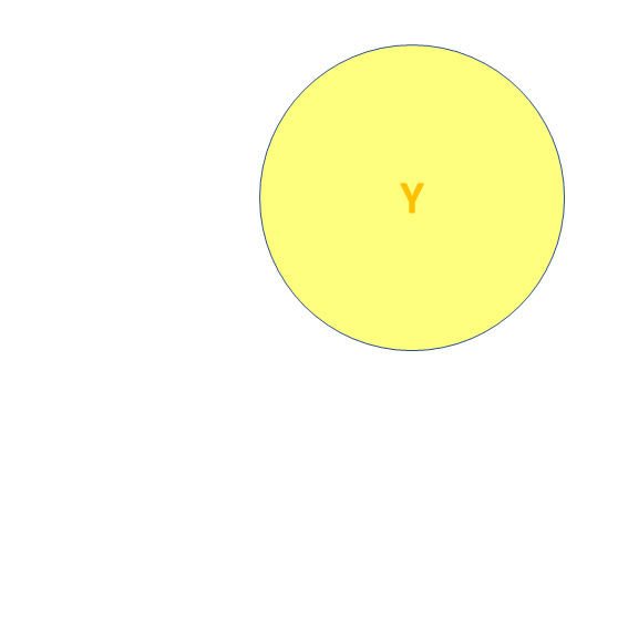
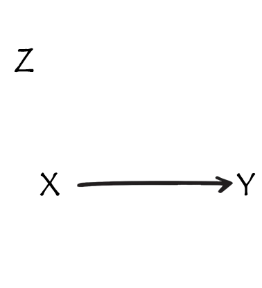
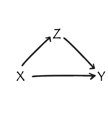
![]() Third variables
Third variables
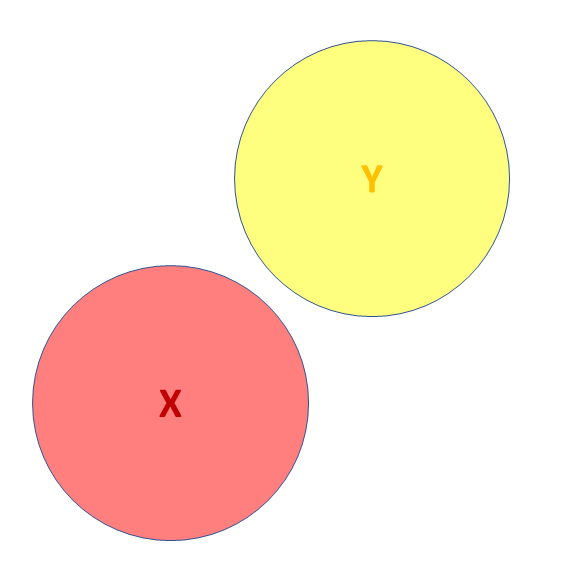
![]() Third variables (2)
Third variables (2)
- X and Y are ‘orthogonal’ (perfectly uncorrelated)
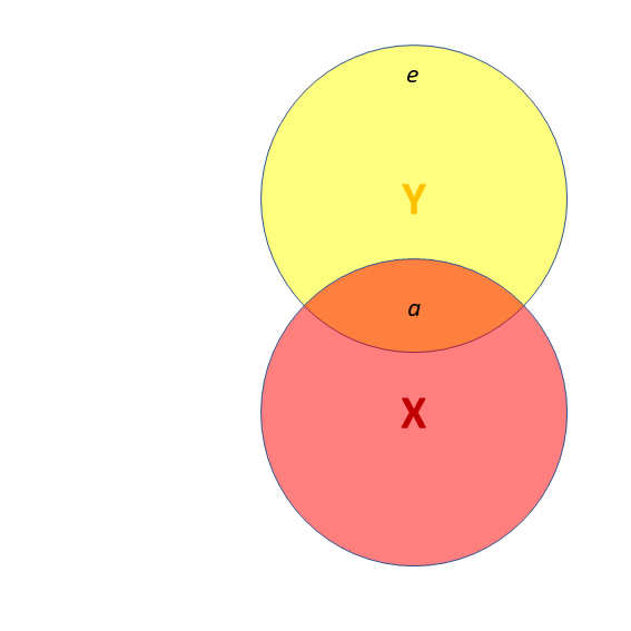
![]() Third variables (3)
Third variables (3)
- X and Y are correlated.
- a = portion of Y’s variance shared with X
- e = portion of Y’s variance unrelated to X
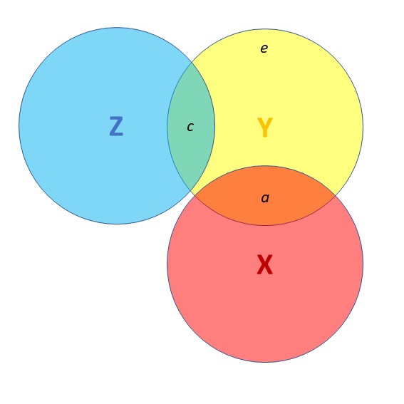
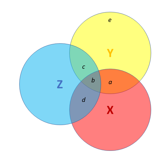
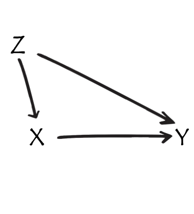
![]() Third variables (4)
Third variables (4)
- X and Y are correlated.
- a = portion of Y’s variance shared with X
- e = portion of Y’s variance unrelated to X
- Z is also related to Y (c)
- Z is orthogonal to X (no overlap)
- relation between X and Y is unaffected (a)
- unexplained variance in Y (e) is reduced, so a:e ratio is greater.
Design is so important! If possible, we could design it so that X and Z are orthogonal (in the long run) by e.g., randomisation.
![]() Third variables (5)
Third variables (5)
- X and Y are correlated.
- Z is also related to Y (c + b)
- Z is related to X (b + d)
Association between X and Y is changed if we adjust for Z (a is smaller than previous slide), because there is a bit (b) that could be attributed to Z instead.
- multiple regression coefficients for X and Z are like areas a and c (scaled to be in terms of ‘per unit change in the predictor’)
- total variance explained by both X and Z is a+b+c
I have control issues..
..and so should you
what do we mean by “control”?
- often quite a vague/nebulous idea
relationship between x and y …
- controlling for z
- accounting for z
- conditional upon z
- holding constant z
- adjusting for z
simple lm(y~x)
what do i do with Z?
Z is… a confounder
Z is… a mediator
Z is… a collider
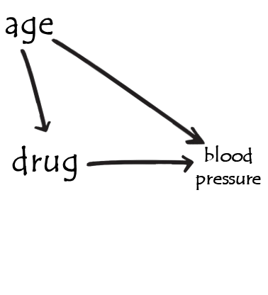
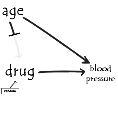
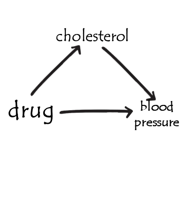
example
example - observational study


example - randomised trial


example - post-treatment variables


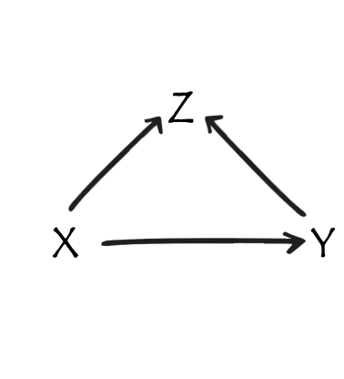
example 2 - colliders

example 2 - colliders
- to play around with this, see https://colliderbias.herokuapp.com/
Multiple Regression
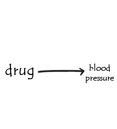
mod1 = lm(BP ~ age + drug, mydata)
summary(mod1)
Call:
lm(formula = BP ~ age + drug, data = mydata)

Residuals:
    Min      1Q  Median      3Q     Max
-14.616  -3.325   0.824   3.709  11.714

Coefficients:
            Estimate Std. Error t value Pr(>|t|)
(Intercept)  62.5566     1.5383    40.7  < 2e-16 ***
age           0.9154     0.0334    27.4  < 2e-16 ***
drugYes      -6.7654     1.1661    -5.8  8.2e-08 ***
---
Signif. codes:  0 '***' 0.001 '**' 0.01 '*' 0.05 '.' 0.1 ' ' 1

Residual standard error: 4.95 on 97 degrees of freedom
Multiple R-squared:  0.898, Adjusted R-squared:  0.896
F-statistic: 427 on 2 and 97 DF, p-value: <2e-16| term | est | interpretation |
|---|---|---|
| (Intercept) | 62.56 | estimated BP when all predictors are zero (age 0, drug = no) |
| age | 0.92 | estimated change in BP when age increases by 1, and drug is held constant |
| drugYes | -6.77 | estimated change in BP between drug = no and drug = yes, holding age constant |
Interactions (2)

summary(lm(y ~ x1 + x2, data = df))Coefficients:
Estimate Std. Error t value Pr(>|t|)
(Intercept) 35.3521 1.0097 35.01 < 2e-16 ***
x1 0.1719 0.0476 3.61 0.00038 ***
x2Level2 -4.3901 0.6740 -6.51 6e-10 ***
summary(lm(y ~ x1 + x2 + x1:x2, data = df))Coefficients:
Estimate Std. Error t value Pr(>|t|)
(Intercept) 30.9050 1.3018 23.74 < 2e-16 ***
x1 0.4095 0.0653 6.27 2.2e-09 ***
x2Level2 3.8539 1.7629 2.19 0.03 *
x1:x2Level2 -0.4510 0.0899 -5.01 1.2e-06 ***Interactions (3)

summary(lm(y ~ x1 + x2, data = df))Coefficients:
Estimate Std. Error t value Pr(>|t|)
(Intercept) -4.009 2.008 -2.00 0.052 .
x1 4.345 0.329 13.22 < 2e-16 ***
x2 3.189 0.402 7.93 3.2e-10 ***
summary(lm(y ~ x1 + x2 + x1:x2, data = df))Coefficients:
Estimate Std. Error t value Pr(>|t|)
(Intercept) 6.004 2.652 2.26 0.028 *
x1 1.347 0.677 1.99 0.053 .
x2 0.561 0.637 0.88 0.383
x1:x2 0.763 0.158 4.83 0.000016 ***Interactions (4)

summary(lm(y ~ x1 + x2 + x1:x2, data = df))Coefficients:
Estimate Std. Error t value Pr(>|t|)
(Intercept) 6.004 2.652 2.26 0.028 *
x1 1.347 0.677 1.99 0.053 .
x2 0.561 0.637 0.88 0.383
x1:x2 0.763 0.158 4.83 0.000016 ***Interactions (5)

summary(lm(y ~ x1 + x2 + x1:x2, data = df))Coefficients:
Estimate Std. Error t value Pr(>|t|)
(Intercept) 6.004 2.652 2.26 0.028 *
x1 1.347 0.677 1.99 0.053 .
x2 0.561 0.637 0.88 0.383
x1:x2 0.763 0.158 4.83 0.000016 ***What is inference?
Null Hypothesis Testing

Null Hypothesis Testing (2)

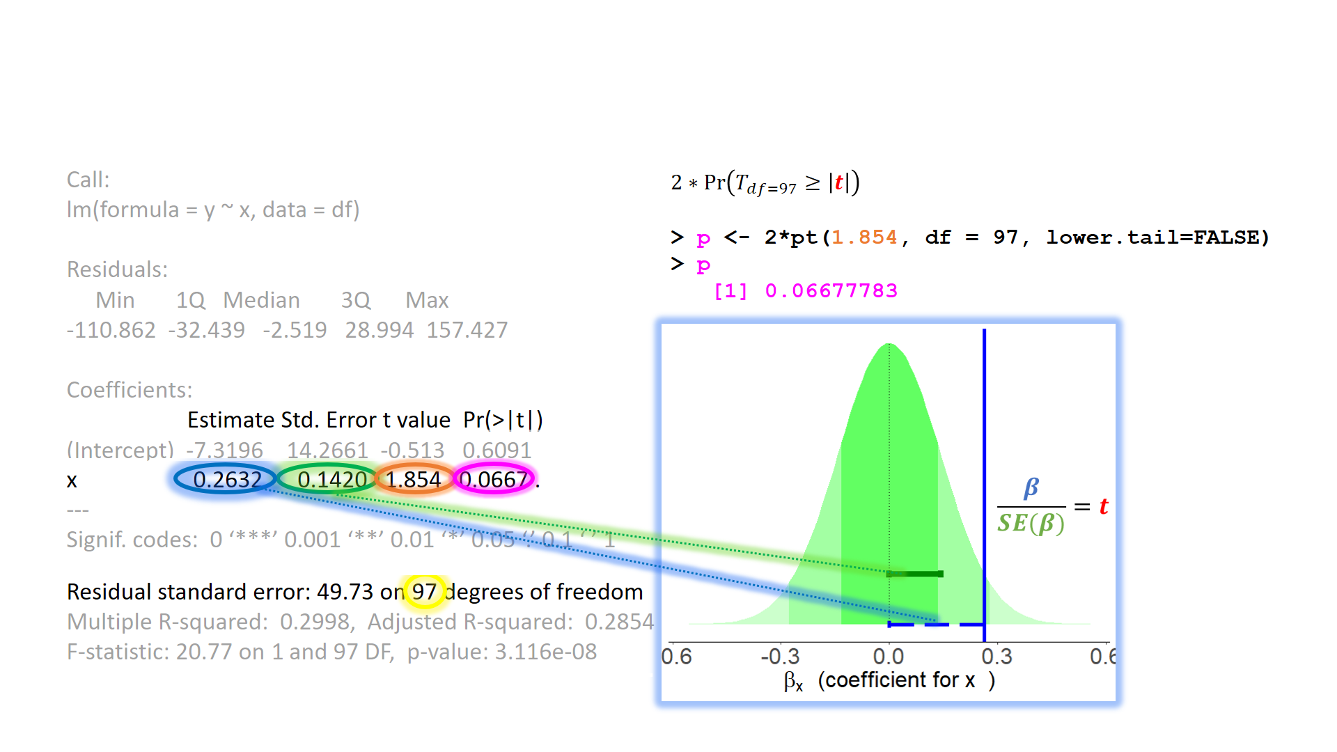
test of individual parameters
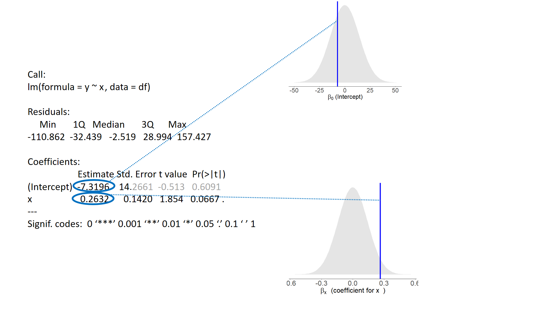
test of individual parameters (2)
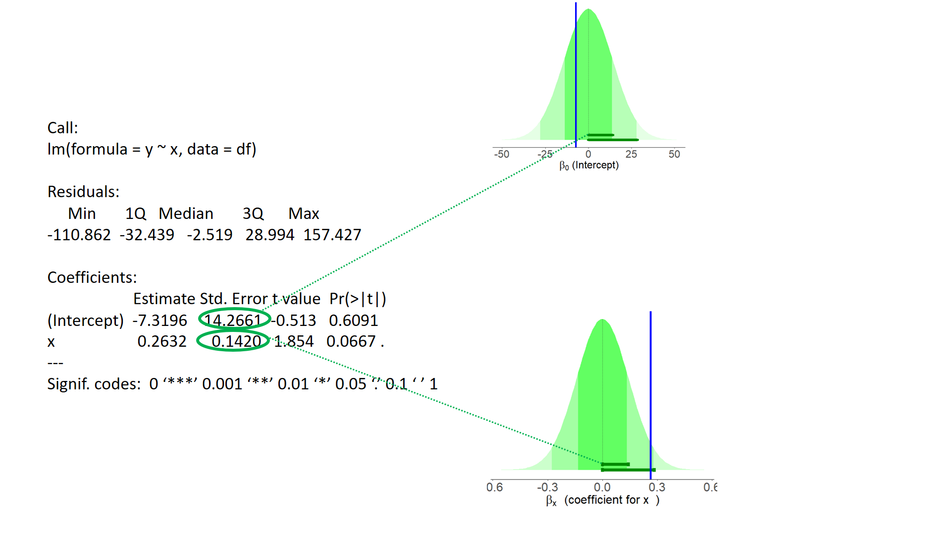
test of individual parameters (3)
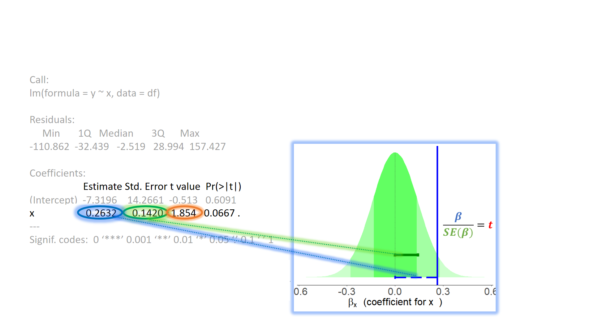
test of individual parameters (4)
Sums of Squares (2)
- \(SS_{total} = \sum^{n}_{i=1}(y_i - \bar y)^2\)
- a+b+c+e
- \(SS_{model} = \sum^{n}_{i=1}(\hat y_i - \bar y)^2\)
- a+b+c
- \(SS_{residual} = \sum^{n}_{i=1}(y_i - \hat y_i)^2\)
- e
\(R^2\)
\(R^2 = \frac{SS_{Model}}{SS_{Total}} = 1 - \frac{SS_{Residual}}{SS_{Total}}\)
mdl <- lm(y ~ 1 + z + x)
summary(mdl)
...
Coefficients:
Estimate Std. Error t value Pr(>|t|)
(Intercept) ... ... ... ...
z ... ... ... ...
x ... ... ... ...
...
...
Multiple R-squared: 0.134, Adjusted R-squared: 0.116
...
tests of multiple parameters
Model comparisons:
m1 <- lm(y ~ 1 + x, data = df)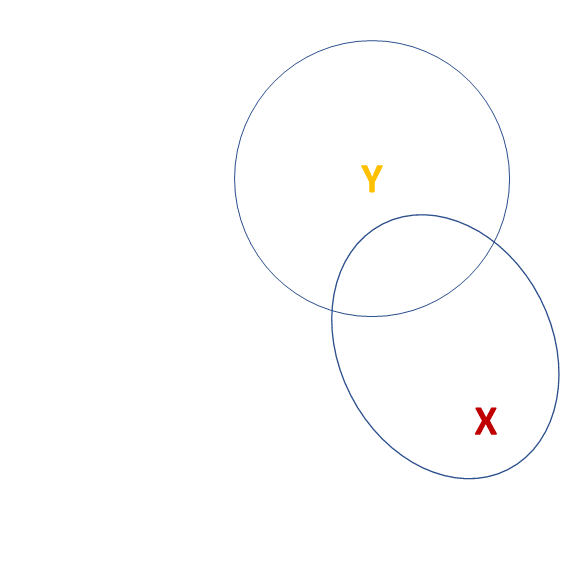
m2 <- lm(y ~ 1 + z + z2 + x, data = df)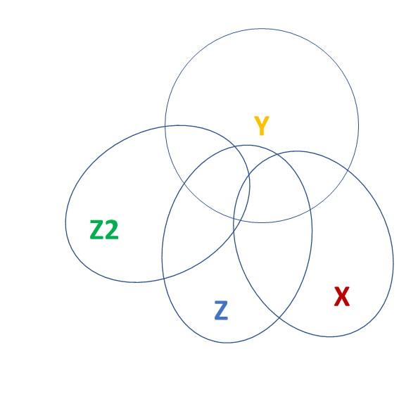
tests of multiple parameters (2)
isolate the improvement in model fit due to inclusion of additional parameters
m1 <- lm(y ~ 1 + x, data = df)
m2 <- lm(y ~ 1 + z + z2 + x, data = df)
anova(m1,m2)
Analysis of Variance Table
Model 1: y ~ 1 + x
Model 2: y ~ 1 + z + z2 + x
Res.Df RSS Df Sum of Sq F Pr(>F)
1 98 1141
2 96 357 2 785 106 <2e-16 ***
---
Signif. codes: 0 '***' 0.001 '**' 0.01 '*' 0.05 '.' 0.1 ' ' 1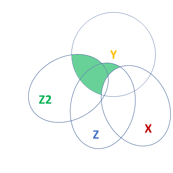
tests of multiple parameters (3)
Test everything in the model all at once by comparing it to a ‘null model’ with no predictors:
m0 <- lm(y ~ 1, data = df)
m2 <- lm(y ~ 1 + z2 + z + x, data = df)
anova(m0,m2)
Analysis of Variance Table
Model 1: y ~ 1
Model 2: y ~ 1 + z2 + z + x
Res.Df RSS Df Sum of Sq F Pr(>F)
1 99 1232
2 96 357 3 875 78.6 <2e-16 ***
---
Signif. codes: 0 '***' 0.001 '**' 0.01 '*' 0.05 '.' 0.1 ' ' 1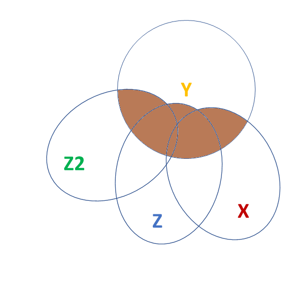
![]() traditional ANOVA/ANCOVA
traditional ANOVA/ANCOVA
This is kind of where traditional “analysis of (co)variance” sits.
There are different ‘types’ of ANOVA..
- Type 1 (“sequential”): tests the addition of each variable entered in to the model, in order
m1 = lm(y ~ z2 + z + x, data = df)
anova(m1)
Analysis of Variance Table
Response: y
Df Sum Sq Mean Sq F value Pr(>F)
z2 1 449 449 120.8 < 2e-16 ***
z 1 322 322 86.7 4.5e-15 ***
x 1 105 105 28.2 7.0e-07 ***
Residuals 96 357 4
---
Signif. codes: 0 '***' 0.001 '**' 0.01 '*' 0.05 '.' 0.1 ' ' 1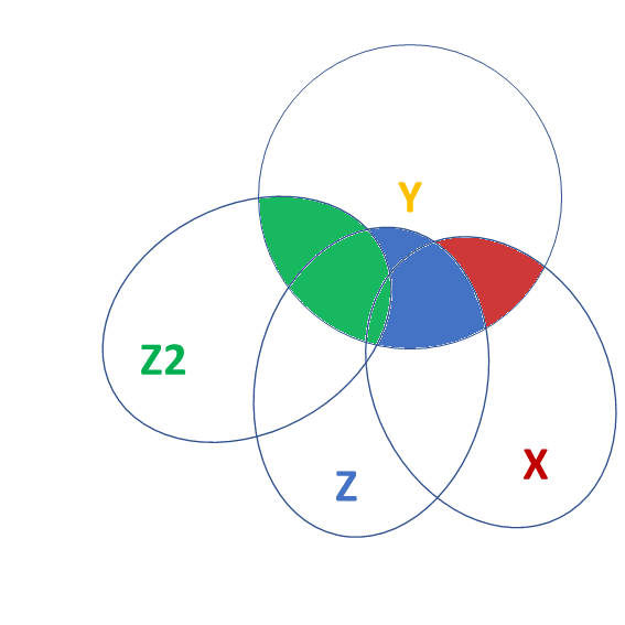
![]() traditional ANOVA/ANCOVA (2)
traditional ANOVA/ANCOVA (2)
This is kind of where traditional “analysis of (co)variance” sits.
There are different ‘types’ of ANOVA..
- Type 3: tests the addition of each variable as if it were the last one entered in to the model:
m1 = lm(y ~ z2 + z + x, data = df)
car::Anova(m1, type="III")
Anova Table (Type III tests)
Response: y
Sum Sq Df F value Pr(>F)
(Intercept) 12041 1 3242.2 < 2e-16 ***
z2 301 1 80.9 2.1e-14 ***
z 352 1 94.8 5.4e-16 ***
x 105 1 28.2 7.0e-07 ***
Residuals 357 96
---
Signif. codes: 0 '***' 0.001 '**' 0.01 '*' 0.05 '.' 0.1 ' ' 1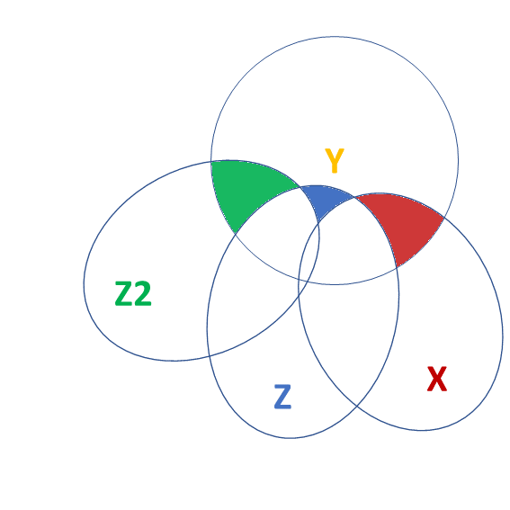
The broader idea
All our work here is in aim of making models of the world (models of how we think the data are generated).
In an ideal world, our model accounts for all the systematic relationships. The leftovers (our residuals) are just random noise.
If our model is mis-specified then our residuals may reflect this.
We check by examining how much “like randomness” the residuals appear to be
We will never know whether our residuals contain only randomness - we can never observe everything!

assumptions
What does randomness look like?
“zero mean and constant variance iid”
mean of the residuals = zero across the predicted values of the model.
spread of residuals is normally distributed and constant across the predicted values of the model.

assumptions (2)
What does randomness look like?
“zero mean and constant variance iid”
mean of the residuals = zero across the predicted values of the model.
spread of residuals is normally distributed and constant across the predicted values of the model.

assumptions (3)
What does randomness look like?
“zero mean and constant variance iid”
mean of the residuals = zero across the predicted values of the model.
spread of residuals is normally distributed and constant across the predicted values of the model.

assumptions (4)
What does randomness look like?
“zero mean and constant variance iid”
mean of the residuals = zero across the predicted values of the model.
spread of residuals is normally distributed and constant across the predicted values of the model.
plot(model)
my_model <- lm(y ~ z + x, data = df)
plot(my_model)
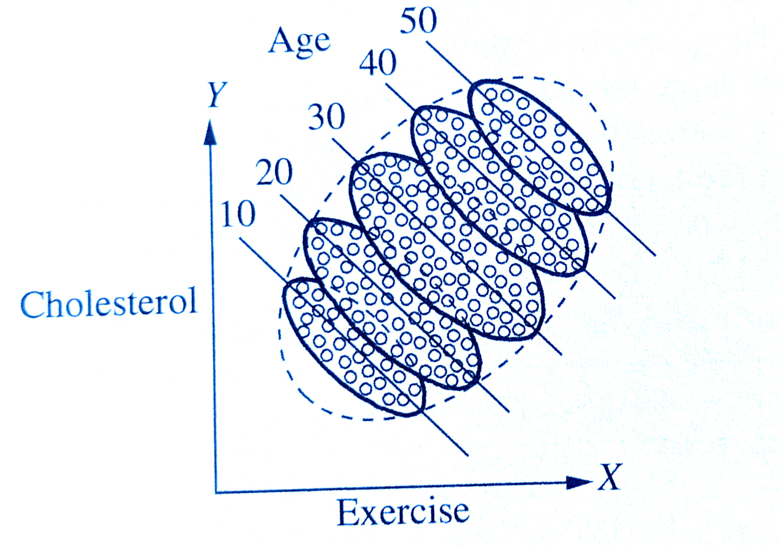
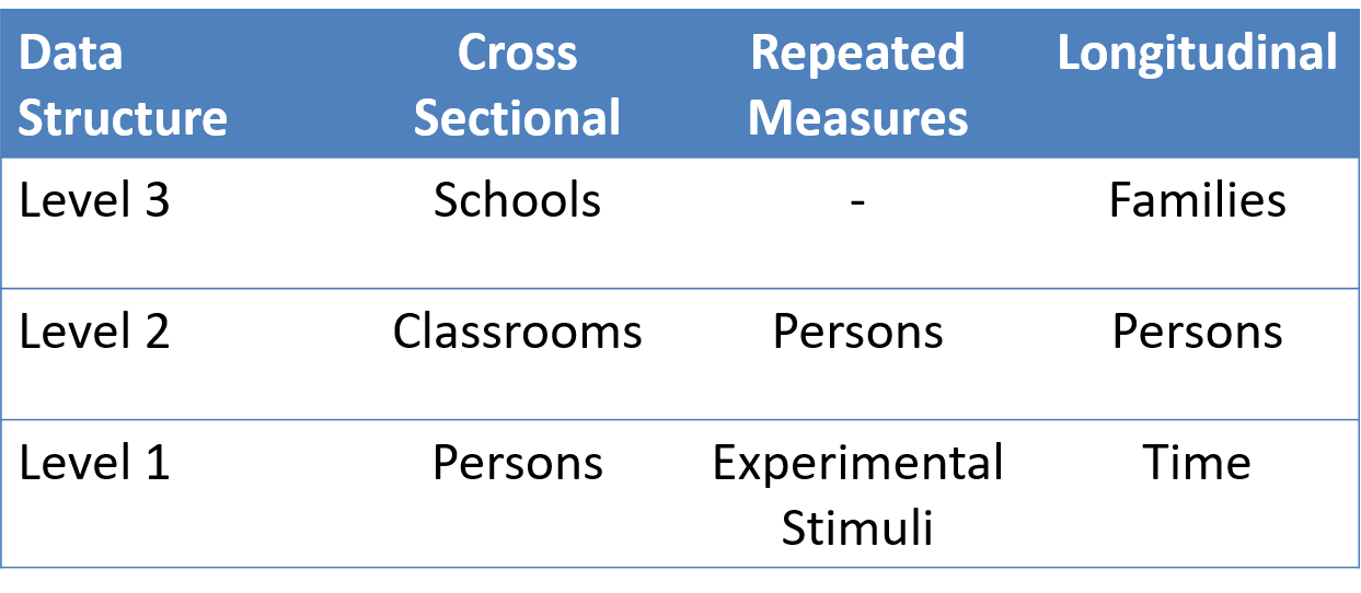
Examples of grouped (‘clustered’) data
children within schools
patients within clinics
observations within individuals
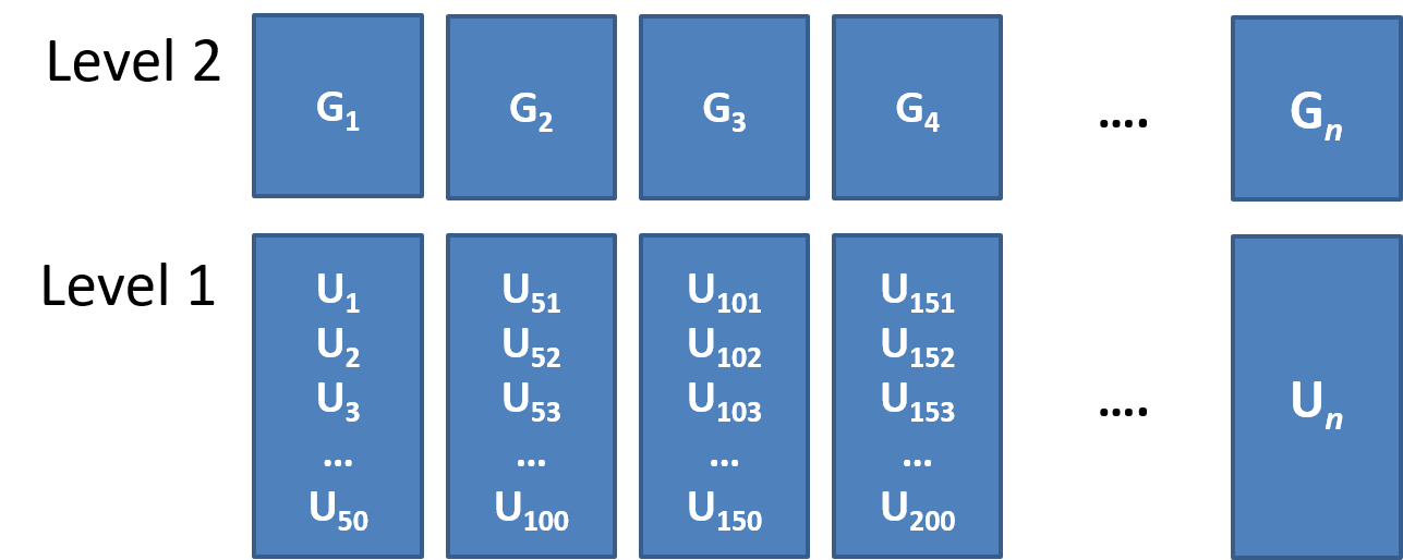
Clusters of clusters
children within classrooms within schools within districts etc…
patients within doctors within hospitals…
time-periods within trials within individuals
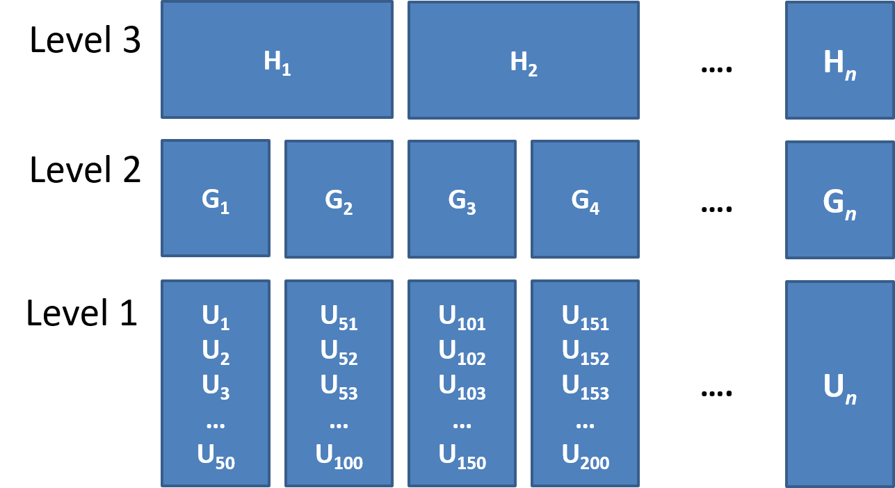
Common study designs
Quantifying clustering
Clustering can be expressed in terms of the expected correlation among the measurements within the same cluster - known as the intra-class correlation coefficient (ICC).
There are various formulations of ICC, but the basic principle = ratio of variance between groups to total variance.
\(\rho = \frac{\sigma^2_{b}}{\sigma^2_{b} + \sigma^2_e} \\ \qquad \\\textrm{Where:} \\ \sigma^2_{b} = \textrm{variance between clusters} \\ \sigma^2_e = \textrm{variance within clusters (residual variance)} \\\)

Long Data = plots by group
group aesthetic
ggplot(longd, aes(x=trial,y=score, group=ID))+
  geom_point(size=4)+
  geom_path()
facet_wrap()
ggplot(longd, aes(x=trial,y=score))+
  geom_point(size=4)+
  geom_path(aes(group=1))+
  facet_wrap(~ID)
Example data
Are older people more satisfied with life? 112 people from 12 different dwellings (cities/towns) in Scotland. Information on their ages and some measure of life satisfaction.
d3 <- read_csv("https://uoepsy.github.io/data/lmm_lifesatscot.csv")
head(d3)
# A tibble: 6 × 4
age lifesat dwelling size
<dbl> <dbl> <chr> <chr>
1 40 31 Aberdeen >100k
2 45 56 Glasgow >100k
3 40 51 Glasgow >100k
4 40 55 Dundee >100k
5 40 41 Dundee >100k
6 55 69 Perth <100k
Ignore it
(Complete pooling)
lm(y ~ 1 + x, data = df)Information from all clusters is pooled together to estimate over x
model <- lm(lifesat ~ 1 + age, data = d3) Estimate Std. Error t value Pr(>|t|)
(Intercept) 30.018 4.889 6.14 1.3e-08 ***
age 0.499 0.118 4.22 5.1e-05 ***
Ignore it
(Complete pooling)
lm(y ~ 1 + x, data = df)Information from all clusters is pooled together to estimate over x
model <- lm(lifesat ~ 1 + age, data = d3) Estimate Std. Error t value Pr(>|t|)
(Intercept) 30.018 4.889 6.14 1.3e-08 ***
age 0.499 0.118 4.22 5.1e-05 ***But residuals are not independent.

Fixed Effects Models
(No pooling)
lm(y ~ cluster + x, data = df)Completely partition out cluster differences in average \(y\).
Treat every cluster as an independent entity.
model <- lm(lifesat ~ 1 + dwelling + age, data = d3) Estimate Std. Error t value Pr(>|t|)
(Intercept) 15.3330 4.1493 3.70 0.00036 ***
dwellingDumfries 8.0741 3.8483 2.10 0.03844 *
dwellingDundee 15.9882 3.8236 4.18 6.3e-05 ***
dwellingDunfermline 26.2600 3.8910 6.75 1.0e-09 ***
dwellingEdinburgh 12.6929 3.8195 3.32 0.00125 **
dwellingFort William 1.3577 3.8999 0.35 0.72849
dwellingGlasgow 18.2906 3.8213 4.79 5.9e-06 ***
dwellingInverness 5.0718 3.8542 1.32 0.19124
... ...
... ...age 0.6047 0.0888 6.81 7.6e-10 ***
---
Fixed Effects Models
(No pooling)
lm(y ~ cluster * x, data = df)Completely partition out cluster differences in \(y \sim x\).
Treat every cluster as an independent entity.
model <- lm(lifesat ~ 1 + dwelling * age, data = d3)Coefficients:
Estimate Std. Error t value Pr(>|t|)
(Intercept) -4.345 8.867 -0.49 0.62532
dwellingDumfries 13.480 14.370 0.94 0.35078
dwellingDundee 59.479 17.650 3.37 0.00112 **
dwellingDunfermline 42.938 17.206 2.50 0.01444 *
... ...age 1.159 0.239 4.84 0.0000054 ***
dwellingDumfries:age -0.206 0.360 -0.57 0.56813
dwellingDundee:age -1.181 0.463 -2.55 0.01243 *
dwellingDunfermline:age -0.486 0.408 -1.19 0.23638
... ...
This week
Tasks
 Complete readings
 Attend your lab and work together on the exercises
 Complete the weekly quiz
Support
 Piazza forum!
 Office hours (see Learn page for details)