A little primer on regression coefficients

Data Analysis for Psychology in R 3

Josiah King

Psychology, PPLS

University of Edinburgh

change in Y for a 1 unit change in X

mod = lm(stress ~ age, data = df)
summary(mod)

Coefficients:
            Estimate Std. Error t value Pr(>|t|)   
(Intercept)  -3.8755     2.3911   -1.62   0.1437   
age           0.2187     0.0633    3.46   0.0086 **
---
Signif. codes:  0 '***' 0.001 '**' 0.01 '*' 0.05 '.' 0.1 ' ' 1

Residual standard error: 3.08 on 8 degrees of freedom
Multiple R-squared:  0.599, Adjusted R-squared:  0.549 
F-statistic: 11.9 on 1 and 8 DF,  p-value: 0.00862

unit level predictions

mod = lm(stress ~ age, data = df)
coef(mod)

(Intercept)         age 
     -3.875       0.219 

Data

# A tibble: 10 × 4
     age exercise therapy  stress
   <dbl>    <dbl>   <dbl>   <dbl>
 1    18        6       0  0.958 
 2    19        6       0  0.0447
 3    20        4       1 -1.81  
 4    33        5       0  7.60  
 5    67        3       1  7.53  
 6    24        1       1  1.61  
 7    37        7       0  6.03  
 8    55        6       0 12.6   
 9    41        4       1  2.60  
10    31        5       1 -0.500 

Predictions

# A tibble: 10 × 1
   prediction
        <dbl>
 1     0.0615
 2     0.280 
 3     0.499 
 4     3.34  
 5    10.8   
 6     1.37  
 7     4.22  
 8     8.15  
 9     5.09  
10     2.90  

unit level counterfactuals

mod = lm(stress ~ age, data = df)
coef(mod)

(Intercept)         age 
     -3.875       0.219 

Data

# A tibble: 10 × 4
     age exercise therapy  stress
   <dbl>    <dbl>   <dbl>   <dbl>
 1    18        6       0  0.958 
 2    19        6       0  0.0447
 3    20        4       1 -1.81  
 4    33        5       0  7.60  
 5    67        3       1  7.53  
 6    24        1       1  1.61  
 7    37        7       0  6.03  
 8    55        6       0 12.6   
 9    41        4       1  2.60  
10    31        5       1 -0.500 

Predictions

# A tibble: 10 × 1
   prediction
        <dbl>
 1     0.0615
 2     0.280 
 3     0.499 
 4     3.34  
 5    10.8   
 6     1.37  
 7     4.22  
 8     8.15  
 9     5.09  
10     2.90  

Counterfactuals

# A tibble: 10 × 3
   term  contrast estimate
   <chr> <chr>       <dbl>
 1 age   +1          0.219
 2 age   +1          0.219
 3 age   +1          0.219
 4 age   +1          0.219
 5 age   +1          0.219
 6 age   +1          0.219
 7 age   +1          0.219
 8 age   +1          0.219
 9 age   +1          0.219
10 age   +1          0.219

unit level counterfactuals

mod = lm(stress ~ therapy, data = df)
coef(mod)

(Intercept)     therapy 
       5.45       -3.57 

Data

# A tibble: 10 × 4
     age exercise therapy  stress
   <dbl>    <dbl>   <dbl>   <dbl>
 1    18        6       0  0.958 
 2    19        6       0  0.0447
 3    20        4       1 -1.81  
 4    33        5       0  7.60  
 5    67        3       1  7.53  
 6    24        1       1  1.61  
 7    37        7       0  6.03  
 8    55        6       0 12.6   
 9    41        4       1  2.60  
10    31        5       1 -0.500 

Predictions

# A tibble: 10 × 1
   prediction
        <dbl>
 1       5.45
 2       5.45
 3       1.89
 4       5.45
 5       1.89
 6       1.89
 7       5.45
 8       5.45
 9       1.89
10       1.89

Counterfactuals

# A tibble: 10 × 3
   term    contrast estimate
   <chr>   <chr>       <dbl>
 1 therapy 1 - 0       -3.57
 2 therapy 1 - 0       -3.57
 3 therapy 1 - 0       -3.57
 4 therapy 1 - 0       -3.57
 5 therapy 1 - 0       -3.57
 6 therapy 1 - 0       -3.57
 7 therapy 1 - 0       -3.57
 8 therapy 1 - 0       -3.57
 9 therapy 1 - 0       -3.57
10 therapy 1 - 0       -3.57

holding constant

mod = lm(stress ~ age + exercise + therapy, data = df)
coef(mod)

(Intercept)         age    exercise     therapy 
      3.087       0.241      -0.908      -6.940 

Data

# A tibble: 10 × 4
     age exercise therapy  stress
   <dbl>    <dbl>   <dbl>   <dbl>
 1    18        6       0  0.958 
 2    19        6       0  0.0447
 3    20        4       1 -1.81  
 4    33        5       0  7.60  
 5    67        3       1  7.53  
 6    24        1       1  1.61  
 7    37        7       0  6.03  
 8    55        6       0 12.6   
 9    41        4       1  2.60  
10    31        5       1 -0.500 

Predictions

# A tibble: 10 × 1
   prediction
        <dbl>
 1      1.98 
 2      2.22 
 3     -2.66 
 4      6.51 
 5      9.58 
 6      1.03 
 7      5.65 
 8     10.9  
 9      2.40 
10     -0.916

Counterfactuals

# A tibble: 10 × 5
     age exercise term    contrast estimate
   <dbl>    <dbl> <chr>   <chr>       <dbl>
 1    18        6 therapy 1 - 0       -6.94
 2    19        6 therapy 1 - 0       -6.94
 3    20        4 therapy 1 - 0       -6.94
 4    33        5 therapy 1 - 0       -6.94
 5    67        3 therapy 1 - 0       -6.94
 6    24        1 therapy 1 - 0       -6.94
 7    37        7 therapy 1 - 0       -6.94
 8    55        6 therapy 1 - 0       -6.94
 9    41        4 therapy 1 - 0       -6.94
10    31        5 therapy 1 - 0       -6.94

interactions

mod = lm(stress ~ age + exercise + therapy + age:therapy, data = df)
coef(mod)

(Intercept)         age    exercise     therapy age:therapy 
      0.220       0.334      -0.932      -1.780      -0.153 

Data

# A tibble: 10 × 4
     age exercise therapy  stress
   <dbl>    <dbl>   <dbl>   <dbl>
 1    18        6       0  0.958 
 2    19        6       0  0.0447
 3    20        4       1 -1.81  
 4    33        5       0  7.60  
 5    67        3       1  7.53  
 6    24        1       1  1.61  
 7    37        7       0  6.03  
 8    55        6       0 12.6   
 9    41        4       1  2.60  
10    31        5       1 -0.500 

Predictions

# A tibble: 10 × 1
   prediction
        <dbl>
 1      0.643
 2      0.977
 3     -1.67 
 4      6.59 
 5      7.76 
 6      1.85 
 7      6.06 
 8     13.0  
 9      2.12 
10     -0.615

Counterfactuals

# A tibble: 10 × 5
     age exercise term    contrast estimate
   <dbl>    <dbl> <chr>   <chr>       <dbl>
 1    18        6 therapy 1 - 0       -4.54
 2    19        6 therapy 1 - 0       -4.69
 3    20        4 therapy 1 - 0       -4.85
 4    33        5 therapy 1 - 0       -6.84
 5    67        3 therapy 1 - 0      -12.1 
 6    24        1 therapy 1 - 0       -5.46
 7    37        7 therapy 1 - 0       -7.45
 8    55        6 therapy 1 - 0      -10.2 
 9    41        4 therapy 1 - 0       -8.07
10    31        5 therapy 1 - 0       -6.53

Think in hypotheticals

mod = lm(stress ~ age, data = df)
summary(mod)

Coefficients:
            Estimate Std. Error t value Pr(>|t|)   
(Intercept)  -3.8755     2.3911   -1.62   0.1437   
age           0.2187     0.0633    3.46   0.0086 **
---
Signif. codes:  0 '***' 0.001 '**' 0.01 '*' 0.05 '.' 0.1 ' ' 1

Residual standard error: 3.08 on 8 degrees of freedom
Multiple R-squared:  0.599, Adjusted R-squared:  0.549 
F-statistic: 11.9 on 1 and 8 DF,  p-value: 0.00862

Think in hypotheticals

mod = lm(stress ~ age, data = df)
summary(mod)

Coefficients:
            Estimate Std. Error t value Pr(>|t|)   
(Intercept)  -3.8755     2.3911   -1.62   0.1437   
age           0.2187     0.0633    3.46   0.0086 **
---
Signif. codes:  0 '***' 0.001 '**' 0.01 '*' 0.05 '.' 0.1 ' ' 1

Residual standard error: 3.08 on 8 degrees of freedom
Multiple R-squared:  0.599, Adjusted R-squared:  0.549 
F-statistic: 11.9 on 1 and 8 DF,  p-value: 0.00862

Think in hypotheticals

mod = lm(stress ~ age, data = df)
summary(mod)

Coefficients:
            Estimate Std. Error t value Pr(>|t|)   
(Intercept)  -3.8755     2.3911   -1.62   0.1437   
age           0.2187     0.0633    3.46   0.0086 **
---
Signif. codes:  0 '***' 0.001 '**' 0.01 '*' 0.05 '.' 0.1 ' ' 1

Residual standard error: 3.08 on 8 degrees of freedom
Multiple R-squared:  0.599, Adjusted R-squared:  0.549 
F-statistic: 11.9 on 1 and 8 DF,  p-value: 0.00862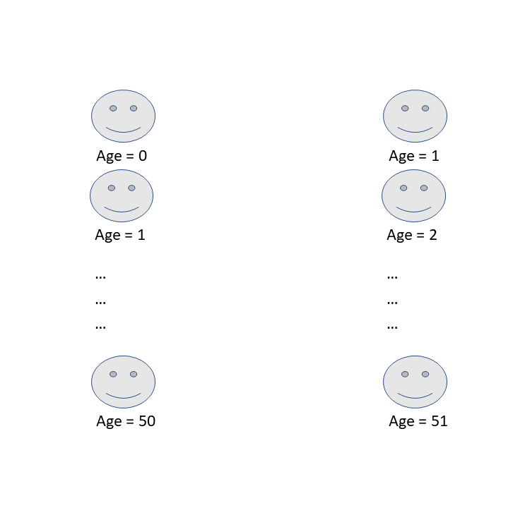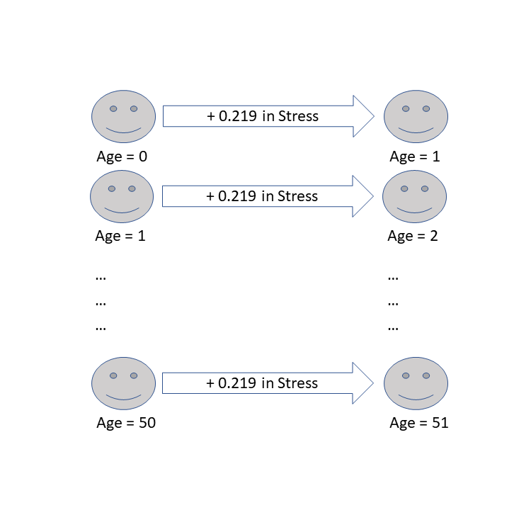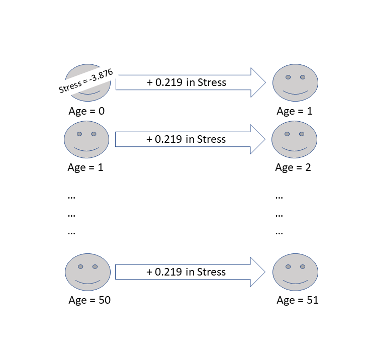

Think in hypotheticals

mod = lm(stress ~ therapy, data = df)
summary(mod)

Coefficients:
            Estimate Std. Error t value Pr(>|t|)  
(Intercept)     5.45       1.99    2.75    0.025 *
therapy        -3.57       2.81   -1.27    0.240  
---
Signif. codes:  0 '***' 0.001 '**' 0.01 '*' 0.05 '.' 0.1 ' ' 1

Residual standard error: 4.44 on 8 degrees of freedom
Multiple R-squared:  0.168, Adjusted R-squared:  0.0637 
F-statistic: 1.61 on 1 and 8 DF,  p-value: 0.24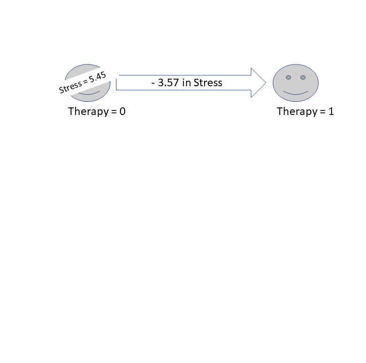

Think in hypotheticals

mod = lm(stress ~ age + exercise + therapy, data = df)
summary(mod)

Coefficients:
            Estimate Std. Error t value Pr(>|t|)    
(Intercept)   3.0874     3.1338    0.99  0.36259    
age           0.2412     0.0334    7.22  0.00036 ***
exercise     -0.9082     0.4817   -1.89  0.10836    
therapy      -6.9398     1.6246   -4.27  0.00525 ** 
---
Signif. codes:  0 '***' 0.001 '**' 0.01 '*' 0.05 '.' 0.1 ' ' 1

Residual standard error: 1.61 on 6 degrees of freedom
Multiple R-squared:  0.918, Adjusted R-squared:  0.877 
F-statistic: 22.3 on 3 and 6 DF,  p-value: 0.00118

Think in hypotheticals

mod = lm(stress ~ age + exercise + therapy, data = df)
summary(mod)

Coefficients:
            Estimate Std. Error t value Pr(>|t|)    
(Intercept)   3.0874     3.1338    0.99  0.36259    
age           0.2412     0.0334    7.22  0.00036 ***
exercise     -0.9082     0.4817   -1.89  0.10836    
therapy      -6.9398     1.6246   -4.27  0.00525 ** 
---
Signif. codes:  0 '***' 0.001 '**' 0.01 '*' 0.05 '.' 0.1 ' ' 1

Residual standard error: 1.61 on 6 degrees of freedom
Multiple R-squared:  0.918, Adjusted R-squared:  0.877 
F-statistic: 22.3 on 3 and 6 DF,  p-value: 0.00118

Think in hypotheticals

mod = lm(stress ~ age + exercise + therapy, data = df)
summary(mod)

Coefficients:
            Estimate Std. Error t value Pr(>|t|)    
(Intercept)   3.0874     3.1338    0.99  0.36259    
age           0.2412     0.0334    7.22  0.00036 ***
exercise     -0.9082     0.4817   -1.89  0.10836    
therapy      -6.9398     1.6246   -4.27  0.00525 ** 
---
Signif. codes:  0 '***' 0.001 '**' 0.01 '*' 0.05 '.' 0.1 ' ' 1

Residual standard error: 1.61 on 6 degrees of freedom
Multiple R-squared:  0.918, Adjusted R-squared:  0.877 
F-statistic: 22.3 on 3 and 6 DF,  p-value: 0.00118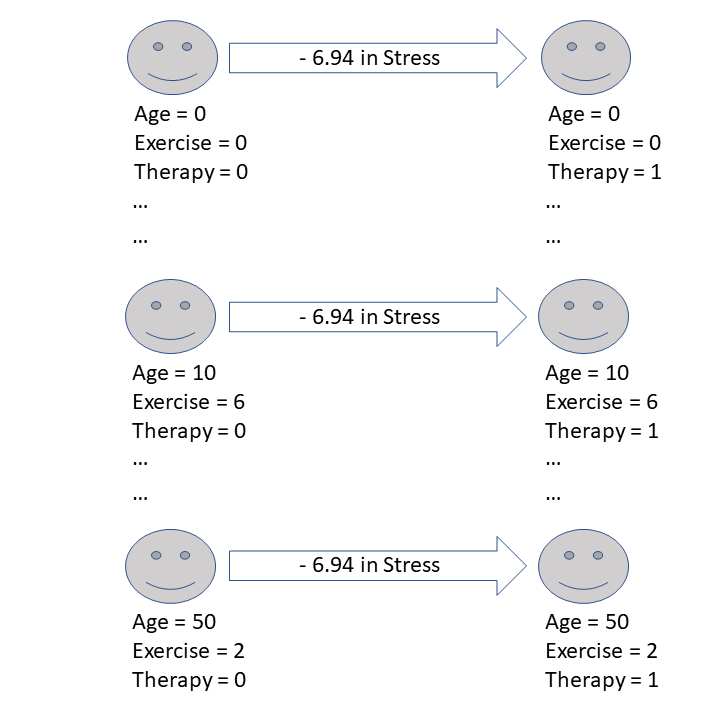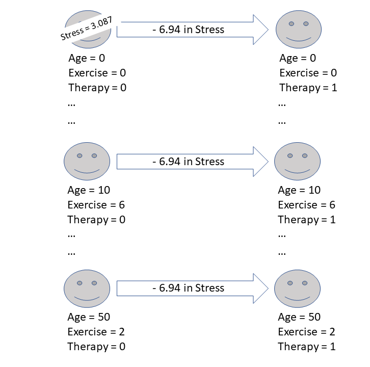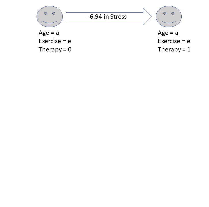

Think in hypotheticals

mod = lm(stress ~ age + exercise + therapy +
           age:therapy, data = df)
summary(mod)

Coefficients:
            Estimate Std. Error t value Pr(>|t|)    
(Intercept)   0.2202     1.4882    0.15   0.8881    
age           0.3340     0.0234   14.28  0.00003 ***
exercise     -0.9316     0.2119   -4.40   0.0070 ** 
therapy      -1.7803     1.2381   -1.44   0.2100    
age:therapy  -0.1533     0.0300   -5.10   0.0038 ** 
---
Signif. codes:  0 '***' 0.001 '**' 0.01 '*' 0.05 '.' 0.1 ' ' 1

Residual standard error: 0.708 on 5 degrees of freedom
Multiple R-squared:  0.987, Adjusted R-squared:  0.976 
F-statistic: 93.1 on 4 and 5 DF,  p-value: 0.00007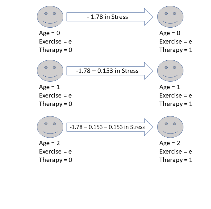

Think in hypotheticals

continuous x continuous interaction

mod = lm(stress ~ age + exercise + n_therapy + 
           age:n_therapy, data = df)
summary(mod)

Coefficients:
              Estimate Std. Error t value Pr(>|t|)    
(Intercept)   -0.01264    1.57115   -0.01  0.99389    
age            0.26691    0.04759    5.61  0.00249 ** 
exercise      -0.42881    0.19850   -2.16  0.08316 .  
n_therapy     -1.24472    0.30802   -4.04  0.00991 ** 
age:n_therapy -0.09348    0.00992   -9.42  0.00023 ***
---
Signif. codes:  0 '***' 0.001 '**' 0.01 '*' 0.05 '.' 0.1 ' ' 1

Residual standard error: 0.883 on 5 degrees of freedom
Multiple R-squared:  0.997, Adjusted R-squared:  0.995 
F-statistic:  429 on 4 and 5 DF,  p-value: 0.00000159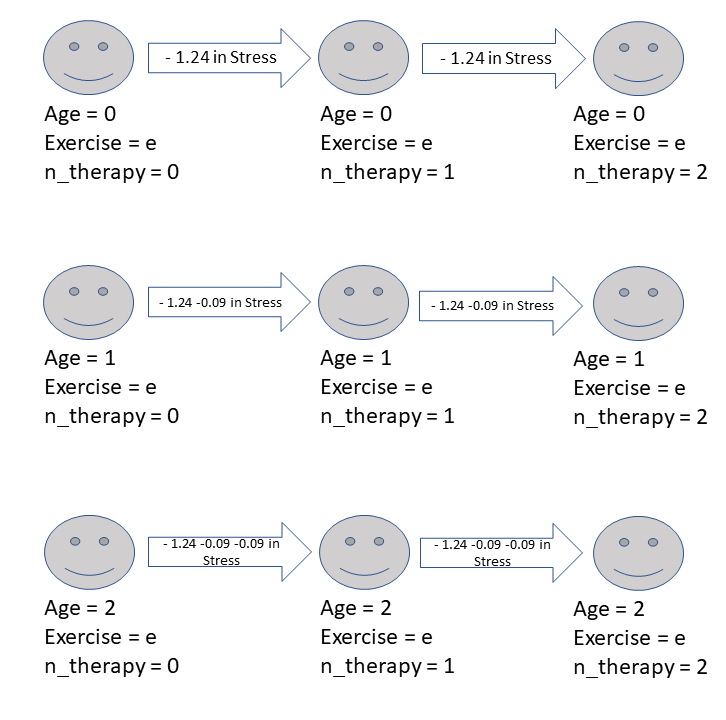

Think in hypotheticals

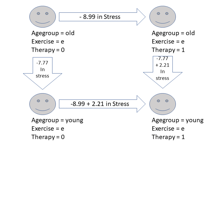
categorical x categorical interaction

mod = lm(stress ~ agegroup + exercise + therapy + 
           agegroup:therapy, data = df)
summary(mod)

Coefficients:
                      Estimate Std. Error t value Pr(>|t|)  
(Intercept)             19.580      6.653    2.94    0.032 *
agegroupyoung           -7.775      2.947   -2.64    0.046 *
exercise                -1.577      0.966   -1.63    0.164  
therapy                 -8.992      4.248   -2.12    0.088 .
agegroupyoung:therapy    2.211      4.061    0.54    0.609  
---
Signif. codes:  0 '***' 0.001 '**' 0.01 '*' 0.05 '.' 0.1 ' ' 1

Residual standard error: 3.11 on 5 degrees of freedom
Multiple R-squared:  0.746, Adjusted R-squared:  0.542 
F-statistic: 3.66 on 4 and 5 DF,  p-value: 0.0935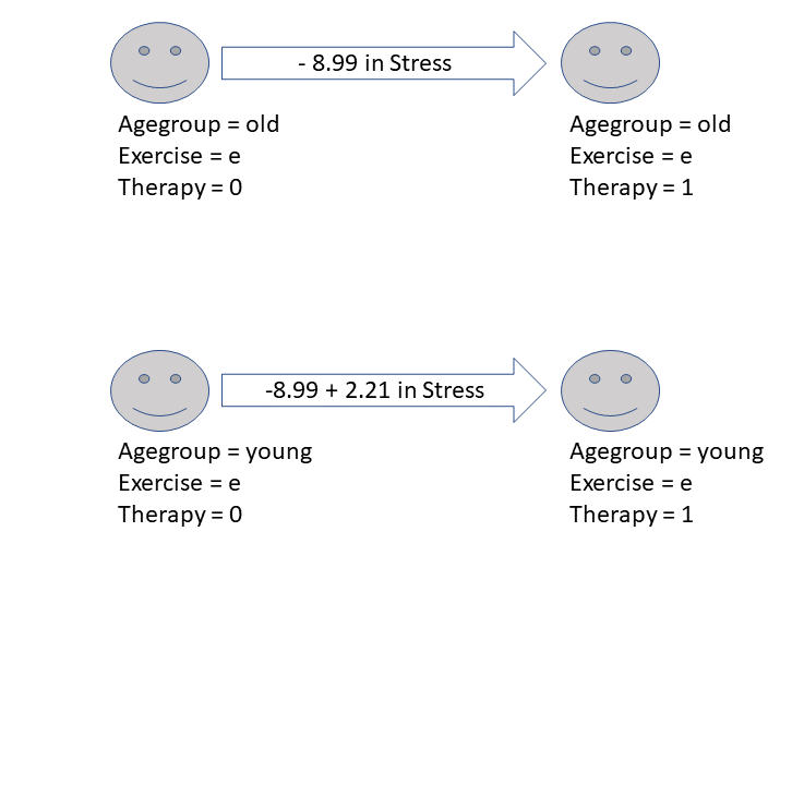

Think in hypotheticals

categorical x categorical interaction

mod = lm(stress ~ agegroup + exercise + therapy + 
           agegroup:therapy, data = df)
summary(mod)

Coefficients:
                      Estimate Std. Error t value Pr(>|t|)  
(Intercept)             19.580      6.653    2.94    0.032 *
agegroupyoung           -7.775      2.947   -2.64    0.046 *
exercise                -1.577      0.966   -1.63    0.164  
therapy                 -8.992      4.248   -2.12    0.088 .
agegroupyoung:therapy    2.211      4.061    0.54    0.609  
---
Signif. codes:  0 '***' 0.001 '**' 0.01 '*' 0.05 '.' 0.1 ' ' 1

Residual standard error: 3.11 on 5 degrees of freedom
Multiple R-squared:  0.746, Adjusted R-squared:  0.542 
F-statistic: 3.66 on 4 and 5 DF,  p-value: 0.0935