| person | y | x | ... |
|---|---|---|---|
| 1 | ... | ... | ... |
| 1 | ... | ... | ... |
| 1 | ... | ... | ... |
| 2 | ... | ... | ... |
| 2 | ... | ... | ... |
| 2 | ... | ... | ... |
| 3 | ... | ... | ... |
| 3 | ... | ... | ... |
| 3 | ... | ... | ... |
Recap!
Data Analysis for Psychology in R 3
Psychology, PPLS
University of Edinburgh
Course Overview
|
multilevel modelling working with group structured data |
regression refresher |
| introducing multilevel models | |
| more complex groupings | |
| centering, assumptions, and diagnostics | |
| recap | |
|
factor analysis working with multi-item measures |
what is a psychometric test? |
| using composite scores to simplify data (PCA) | |
| uncovering underlying constructs (EFA) | |
| more EFA | |
| recap & exam prep |
This week
- Lec1: Recap of core concepts
- Lec2: Exam prep session
- Lab: Mock Exam Qs
Broad ideas
multivariate
mixed models/multi-level models
- multiple values per cluster
- each value is an observation
pscyhometrics
- multiple values (\(y1, ..., y_k\)) representing the same construct
- the set of values is “an observation” of Y
| person | y1 | y2 | y3 | ... |
|---|---|---|---|---|
| 1 | ... | ... | ... | ... |
| 2 | ... | ... | ... | ... |
| 3 | ... | ... | ... | ... |
| ... | ... | ... | ... | ... |
two questions
- Q: To do anything with [construct Y], how do we get one number to represent an observation of Y?
- is one number enough - are \(y1,y2,...,yk\) really unidimensional?
- Q: How does [set of scores \(y1,y2,...,yk\)] get at [construct Y]?
- is it a reliable measure?
- are the variables equally representative?
- is there just one dimension to Y or are there multiple?
scoring multi-item measures
scale scores
add ’em all up, you’ve got Y
- clinically ‘meaningful’?
- but only ‘meaningful’ if underlying model holds (which it almost definitely doesn’t!)
dimension reduction
identify dimensions that capture how people co-vary across across the items
PCA: reduce to set of orthogonal dimensions sequentially capturing most variability
FA: develop theoretical model of underlying dimensions (possibly correlated) that explain variability in items
understanding multi-item measures
dimension reduction
identify dimensions that capture how people co-vary across across the items
- PCA: reduce to set of orthogonal dimensions sequentially capturing most variability
- FA: develop theoretical model of underlying dimensions (possibly correlated) that explain variability in items
understanding multi-item measures
\[ \begin{align} \text{Outcome} &=& \text{Model} &\quad + \quad& \text{Error} \\ \quad \\ \text{observed correlation} &=& \text{factor loadings and} &\quad + \quad& \text{unique variance for} \\ \text{matrix of items}& &\text{factor correlations} &\quad + \quad& \text{each item} \\ \end{align} \]
dimension reduction
the idea
Correlations between times can reflect the extent to which items ‘measure the same thing’
If items all measure completely different things
If items all measure the same thing perfectly
the idea
Correlations between times can reflect the extent to which items ‘measure the same thing’
If items all measure completely different things
If items all measure the same thing (imperfectly)
the idea
- people vary in lots of ways over k variables
- capture the ways in which people vary.
the idea
- people vary in lots of ways over k variables
- capture the ways in which people vary.
| y1 | y2 | y3 | y4 | y5 | y6 | |
|---|---|---|---|---|---|---|
| y1 | 1.00 | 0.60 | 0.63 | 0.15 | 0.14 | 0.26 |
| y2 | 0.60 | 1.00 | 0.61 | 0.19 | 0.12 | 0.21 |
| y3 | 0.63 | 0.61 | 1.00 | 0.27 | 0.27 | 0.30 |
| y4 | 0.15 | 0.19 | 0.27 | 1.00 | 0.72 | 0.68 |
| y5 | 0.14 | 0.12 | 0.27 | 0.72 | 1.00 | 0.65 |
| y6 | 0.26 | 0.21 | 0.30 | 0.68 | 0.65 | 1.00 |
dimension reduction - what do we get?
broadly:
relationships between observed variables and the dimensions
amount of variance explained by each dimension
loadings
Principal Components Analysis
Call: principal(r = somedata, nfactors = 6, rotate = "none")
Standardized loadings (pattern matrix) based upon correlation matrix
    PC1   PC2   PC3   PC4   PC5   PC6 h2       u2 com
y1 0.64  0.59 -0.41  0.08  0.25 -0.08  1 -4.4e-16 3.1
y2 0.62  0.59  0.39  0.30  0.03  0.12  1 -2.2e-16 3.3
y3 0.72  0.48  0.05 -0.43 -0.25 -0.04  1 -8.9e-16 2.8
y4 0.74 -0.52  0.17  0.04  0.07 -0.39  1  1.1e-16 2.5
y5 0.71 -0.54  0.06 -0.20  0.27  0.29  1  2.2e-16 2.8
y6 0.76 -0.42 -0.24  0.25 -0.32  0.12  1  2.2e-16 2.6
...
\(\text{loading}\) = cor(item, dimension)
loadings
Principal Components Analysis
Call: principal(r = somedata, nfactors = 6, rotate = "none")
Standardized loadings (pattern matrix) based upon correlation matrix
    PC1   PC2   PC3   PC4   PC5   PC6 h2       u2 com
y1 0.64  0.59 -0.41  0.08  0.25 -0.08  1 -4.4e-16 3.1
y2 0.62  0.59  0.39  0.30  0.03  0.12  1 -2.2e-16 3.3
y3 0.72  0.48  0.05 -0.43 -0.25 -0.04  1 -8.9e-16 2.8
y4 0.74 -0.52  0.17  0.04  0.07 -0.39  1  1.1e-16 2.5
y5 0.71 -0.54  0.06 -0.20  0.27  0.29  1  2.2e-16 2.8
y6 0.76 -0.42 -0.24  0.25 -0.32  0.12  1  2.2e-16 2.6
...
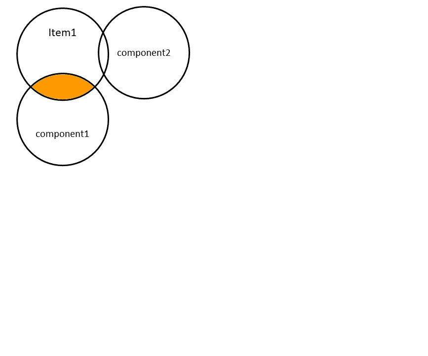
\(\text{loading}^2\) = \(R^2\) from lm(item ~ dimension)
SSloadings & Variance Accounted for
Principal Components Analysis
Call: principal(r = somedata, nfactors = 6, rotate = "none")
Standardized loadings (pattern matrix) based upon correlation matrix
    PC1   PC2   PC3   PC4   PC5   PC6 h2       u2 com
y1 0.64  0.59 -0.41  0.08  0.25 -0.08  1 -4.4e-16 3.1
y2 0.62  0.59  0.39  0.30  0.03  0.12  1 -2.2e-16 3.3
y3 0.72  0.48  0.05 -0.43 -0.25 -0.04  1 -8.9e-16 2.8
y4 0.74 -0.52  0.17  0.04  0.07 -0.39  1  1.1e-16 2.5
y5 0.71 -0.54  0.06 -0.20  0.27  0.29  1  2.2e-16 2.8
y6 0.76 -0.42 -0.24  0.25 -0.32  0.12  1  2.2e-16 2.6

                       PC1  PC2  PC3  PC4  PC5  PC6
SS loadings           2.95 1.66 0.42 0.39 0.31 0.27
...
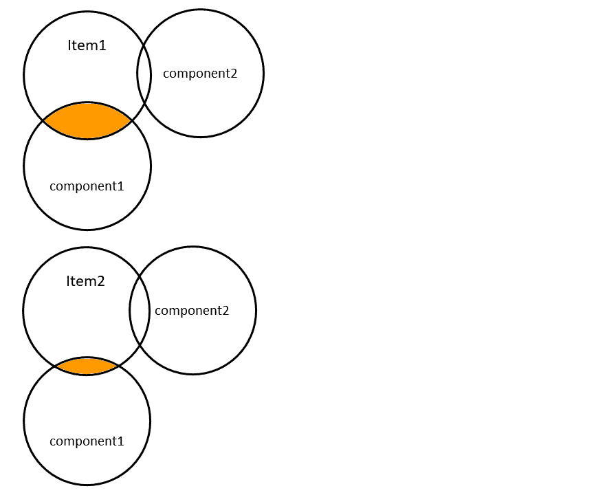
\(\text{SSloading}\) = “sum of squared loadings”
\(R^2\) from lm(item1 ~ dimension) + \(R^2\) from lm(item2 ~ dimension) + \(R^2\) from lm(item3 ~ dimension) + ….
SSloadings & Variance Accounted for
Principal Components Analysis
Call: principal(r = somedata, nfactors = 6, rotate = "none")
Standardized loadings (pattern matrix) based upon correlation matrix
    PC1   PC2   PC3   PC4   PC5   PC6 h2       u2 com
y1 0.64  0.59 -0.41  0.08  0.25 -0.08  1 -4.4e-16 3.1
y2 0.62  0.59  0.39  0.30  0.03  0.12  1 -2.2e-16 3.3
y3 0.72  0.48  0.05 -0.43 -0.25 -0.04  1 -8.9e-16 2.8
y4 0.74 -0.52  0.17  0.04  0.07 -0.39  1  1.1e-16 2.5
y5 0.71 -0.54  0.06 -0.20  0.27  0.29  1  2.2e-16 2.8
y6 0.76 -0.42 -0.24  0.25 -0.32  0.12  1  2.2e-16 2.6

                       PC1  PC2  PC3  PC4  PC5  PC6
SS loadings           2.95 1.66 0.42 0.39 0.31 0.27
Proportion Var        0.49 0.28 0.07 0.07 0.05 0.04
Cumulative Var        0.49 0.77 0.84 0.90 0.96 1.00
...
Total variance = nr of items (e.g., explaining everything would have \(R^2=1\) for each item)
\(\frac{\text{SSloading}}{\text{nr items}}\) = variance accounted for by each dimension
PCA
Principal Components Analysis
Call: principal(r = somedata, nfactors = 6, rotate = "none")
Standardized loadings (pattern matrix) based upon correlation matrix
    PC1   PC2   PC3   PC4   PC5   PC6 h2       u2 com
y1 0.64  0.59 -0.41  0.08  0.25 -0.08  1 -4.4e-16 3.1
y2 0.62  0.59  0.39  0.30  0.03  0.12  1 -2.2e-16 3.3
y3 0.72  0.48  0.05 -0.43 -0.25 -0.04  1 -8.9e-16 2.8
y4 0.74 -0.52  0.17  0.04  0.07 -0.39  1  1.1e-16 2.5
y5 0.71 -0.54  0.06 -0.20  0.27  0.29  1  2.2e-16 2.8
y6 0.76 -0.42 -0.24  0.25 -0.32  0.12  1  2.2e-16 2.6

                       PC1  PC2  PC3  PC4  PC5  PC6
SS loadings           2.95 1.66 0.42 0.39 0.31 0.27
Proportion Var        0.49 0.28 0.07 0.07 0.05 0.04
Cumulative Var        0.49 0.77 0.84 0.90 0.96 1.00
...- Essentially a calculation
- Re-expresses \(k\) items as \(k\) orthogonal dimensions (components) the sequentially capture most variance
- We decide to keep a subset of components based on:
- how many things we ultimately want
- how much variance is captured
- Theory about what the dimensions are doesn’t really matter
conceptual shift to EFA
Factor Analysis using method =  ml
Call: fa(r = somedata, nfactors = 2, rotate = "oblimin", fm = "ml")
Standardized loadings (pattern matrix) based upon correlation matrix
     ML1   ML2   h2   u2 com
y1 -0.04  0.81 0.63 0.37   1
y2 -0.04  0.77 0.58 0.42   1
y3  0.10  0.77 0.64 0.36   1
y4  0.87 -0.02 0.74 0.26   1
y5  0.85 -0.04 0.70 0.30   1
y6  0.76  0.09 0.63 0.37   1

                       ML1  ML2
SS loadings           2.07 1.85
Proportion Var        0.34 0.31
Cumulative Var        0.34 0.65
Proportion Explained  0.53 0.47
Cumulative Proportion 0.53 1.00
...- Is a model (set of parameters are estimated)
“variance captured by components”- “variance explained by factors”
- We choose a model that best explains our observed relationships
- numerically (i.e. distinct factors that each capture something shared across items)
- theoretically (i.e. factors make sense)
- in psych, PCA is often used as a type of EFA (components are interpreted meaningfully, considered as ‘explanatory’, and sometimes rotated! In most other fields, PCA is pure reduction
EFA compared to PCA
Pretty much the same idea: captures relations between items and dimensions, and variance explained by dimensions
BUT - the aim is to explain, not just reduce
- best explanation might not be two orthogonal dimensions
- rotations allow factors to be correlated
EFA output and rotations
observed covariance = factors + unique item variance
- think of a rotation as a transformation applied to the factors
- it doesn’t change the numerical ‘fit’ of the model, but it changes the interpretation
EFA output and rotations
Loadings:
   ML1   ML2
y1 0.209 0.793
y2 0.205 0.762
y3 0.335 0.796
y4 0.860 0.254
y5 0.835 0.225
y6 0.788 0.325

                 ML1   ML2
SS loadings    2.255 2.065
Proportion Var 0.376 0.344
Cumulative Var 0.376 0.720
...
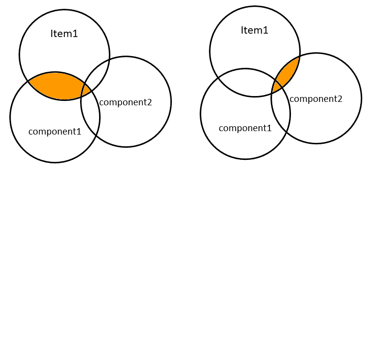
Structure matrix show cor(item, factor)
- but dimensions are now correlated
EFA output and rotations
Factor Analysis using method =  ml
Call: fa(r = somedata, nfactors = 2, rotate = "oblimin", fm = "ml")
Standardized loadings (pattern matrix) based upon correlation matrix
     ML1   ML2   h2   u2 com
y1 -0.04  0.81 0.63 0.37   1
y2 -0.04  0.77 0.58 0.42   1
y3  0.10  0.77 0.64 0.36   1
y4  0.87 -0.02 0.74 0.26   1
y5  0.85 -0.04 0.70 0.30   1
y6  0.76  0.09 0.63 0.37   1

                       ML1  ML2
SS loadings           2.07 1.85
Proportion Var        0.34 0.31
Cumulative Var        0.34 0.65
Proportion Explained  0.53 0.47
Cumulative Proportion 0.53 1.00

 With factor correlations of
     ML1  ML2
ML1 1.00 0.31
ML2 0.31 1.00

...
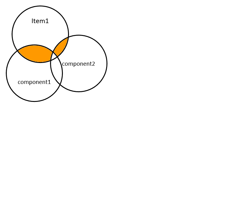
Pattern matrix shows:
- Loadings:
- like
lm(item ~ F1 + F2) |> coef()
- like
EFA output and rotations
Factor Analysis using method =  ml
Call: fa(r = somedata, nfactors = 2, rotate = "oblimin", fm = "ml")
Standardized loadings (pattern matrix) based upon correlation matrix
     ML1   ML2   h2   u2 com
y1 -0.04  0.81 0.63 0.37   1
y2 -0.04  0.77 0.58 0.42   1
y3  0.10  0.77 0.64 0.36   1
y4  0.87 -0.02 0.74 0.26   1
y5  0.85 -0.04 0.70 0.30   1
y6  0.76  0.09 0.63 0.37   1

                       ML1  ML2
SS loadings           2.07 1.85
Proportion Var        0.34 0.31
Cumulative Var        0.34 0.65
...
Pattern matrix shows:
- Communalities & Uniqueness:
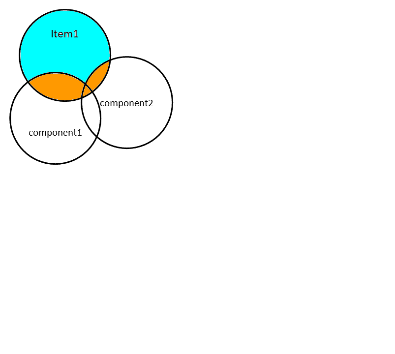
- \(R^2\) and \(1-R^2\) from
lm(item ~ F1 + F2)
- \(R^2\) and \(1-R^2\) from
EFA output and rotations
Factor Analysis using method =  ml
Call: fa(r = somedata, nfactors = 2, rotate = "oblimin", fm = "ml")
Standardized loadings (pattern matrix) based upon correlation matrix
     ML1   ML2   h2   u2 com
y1 -0.04  0.81 0.63 0.37   1
y2 -0.04  0.77 0.58 0.42   1
y3  0.10  0.77 0.64 0.36   1
y4  0.87 -0.02 0.74 0.26   1
y5  0.85 -0.04 0.70 0.30   1
y6  0.76  0.09 0.63 0.37   1

                       ML1  ML2
SS loadings           2.07 1.85
Proportion Var        0.34 0.31
Cumulative Var        0.34 0.65
...
SSloadings
- in the structure and the pattern matrix, SSloadings are simply summing the squared values of the columns.
Variance Accounted For
- trickier because of factor correlations:
getting scores
- PCA & EFA allow us to get weighted scores
EFA is an explanatory model
- Q: To do anything with [construct Y], how do we get one number to represent an observation of Y?
- is one number enough - are \(y1,y2,...,yk\) really unidimensional?
- Q: How does [set of scores \(y1,y2,...,yk\)] get at [construct Y]?
- is it a reliable measure?
- are the variables equally representative?
- is there just one dimension to Y or are there multiple?
Q: is it reliable?
Am I consistently actually measuring a thing?
- this is all necessary because of measurement error
- with perfect measurement we would only need one variable
- more measurement error >>> lower reliability
- sometimes i’m scored too high, sometimes too low, etc.. noise!
- Reliability is a precursor to validity; a test cannot be valid if it is not reliable.
- lots of different ways to investigate reliability
- test-retest
- parallel forms
- inter-rater
- internal consistency (i.e. within a scale)
- \(\alpha\) (assumes equal loadings)
- \(\omega\) (based on factor model)
Validity
Am I measuring the thing I think I’m measuring?
- Lots of different types:
- face validity
- content/construct validity
- convergent validity
- discriminant validity
- predictive validity
- some can be assessed through expected relations with other constructs
- some are assessed through studying the measurement scale and how it is interpreted