Regression Refresh

Data Analysis for Psychology in R 3

Josiah King

Psychology, PPLS

University of Edinburgh

Announcements

• Please check the Learn page for the Course Introduction video!

• Please make sure you install (or update) R and Rstudio (see instructions on Learn)

Course Overview

multilevel modelling working with group structured data	regression refresher
	introducing multilevel models
	more complex groupings
	centering, assumptions, and diagnostics
	recap
factor analysis working with multi-item measures	what is a psychometric test?
	using composite scores to simplify data (PCA)
	uncovering underlying constructs (EFA)
	more EFA
	recap

This week

• The (generalised) linear model
  • model structures (multiple predictors, interactions, link functions)
  • inference (coefficients and model comparisons)
  • assumptions
• introduction to group-structured data
  • what it looks like
  • what we can do with our current tools

Model Structures

Models

deterministic

given the same input, deterministic functions return exactly the same output

• area of sphere = \(4\pi r^2\)

• height of fall = \(1/2 g t^2\)

statistical

\[ \color{red}{\textrm{outcome}} \color{black}{=} \color{blue}{(\textrm{model})} + \color{black}{\textrm{error}} \]

• handspan = height + randomness

• cognitive test score = age + premorbid IQ + … + randomness

The Linear Model

\[ \begin{align} \color{red}{\textrm{outcome}} & = \color{blue}{(\textrm{model})} + \textrm{error} \\ \qquad \\ \qquad \\ \color{red}{y_i} & = \color{blue}{b_0 \cdot{} 1 + b_1 \cdot{} x_i} + \varepsilon_i \\ \qquad \\ & \text{where } \varepsilon_i \sim N(0, \sigma) \text{ independently} \\ \end{align} \]

The Linear Model

Our proposed model of the world:

\(\color{red}{y_i} = \color{blue}{b_0 \cdot{} 1 + b_1 \cdot{} x_i} + \varepsilon_i\)

The Linear Model

Our model \(\hat{\textrm{f}}\textrm{itted}\) to some data:

\(\hat{y}_i = \color{blue}{\hat b_0 \cdot{} 1 + \hat b_1 \cdot{} x_i}\)

For the \(i^{th}\) observation:

• \(\color{red}{y_i}\) is the value we observe for \(x_i\)
  
• \(\hat{y}_i\) is the value the model predicts for \(x_i\)
  
• \(\color{red}{y_i} = \hat{y}_i + \hat\varepsilon_i\)

An example

Our model \(\hat{\textrm{f}}\textrm{itted}\) to some data:

\(\color{red}{y_i} = \color{blue}{5 \cdot{} 1 + 2 \cdot{} x_i} + \hat\varepsilon_i\)

For the observation \(x_i = 1.2, \; y_i = 9.9\):

\[ \begin{align} \color{red}{9.9} & = \color{blue}{5 \cdot{}} 1 + \color{blue}{2 \cdot{}} 1.2 + \hat\varepsilon_i \\ & = 7.4 + \hat\varepsilon_i \\ & = 7.4 + 2.5 \\ \end{align} \]

minimizing residuals

Categorical Predictors

y	x
7.99	Category1
4.73	Category0
3.66	Category0
3.41	Category0
5.75	Category1
5.66	Category0
...	...

Multiple Regression

More than one predictor?

\(\color{red}{y} = \color{blue}{b_0 \cdot{} 1 + b_1 \cdot{} x_1 + \, ... \, + b_k \cdot x_k} + \varepsilon\)

minimizing residuals

I’ve stopped showing the \(i\)’s for now because we start to have more subscripts, but for any individual \(i\), our model is

\(\color{red}{y_i} = \color{blue}{b_0 \cdot{} 1 + b_1 \cdot{} x_{1i} + \, ... \, + b_k \cdot x_{ki}} + \varepsilon_i\)

Multiple Regression

mod1 <- lm(y ~ x1 + x2, data = mydata)
summary(mod1)

Call:
lm(formula = y ~ x1 + x2, data = mydata)

Residuals:
   Min     1Q Median     3Q    Max 
-28.85  -6.27  -0.19   6.97  26.05 

Coefficients:
            Estimate Std. Error t value Pr(>|t|)    
(Intercept)   20.372      1.124   18.12   <2e-16 ***
x1             1.884      1.295    1.46   0.1488    
x2             2.042      0.624    3.28   0.0015 ** 
---
Signif. codes:  0 '***' 0.001 '**' 0.01 '*' 0.05 '.' 0.1 ' ' 1

Residual standard error: 11.2 on 97 degrees of freedom
Multiple R-squared:  0.135, Adjusted R-squared:  0.118 
F-statistic:  7.6 on 2 and 97 DF,  p-value: 0.00086

term	est	interpretation
(Intercept)	20.37	estimated y when all predictors are zero/reference level
x1	1.88	estimated change in y when x1 increases by 1, and all other predictors are held constant
x2	2.04	estimated change in y when x2 increases by 1, and all other predictors are held constant

• coefficients now interpreted with “holding constant”

associations in regression

TANGENT.
why useful?

visual is for learning only - intution building.

associations in regression

• X and Y are ‘orthogonal’ (perfectly uncorrelated)

associations in regression

• X and Y are correlated.
  • a = portion of Y’s variance shared with X
  • e = portion of Y’s variance unrelated to X

• SIGNAL / NOISE
  
• a/e

associations in regression

• X and Y are correlated.
  • a = portion of Y’s variance shared with X
  • e = portion of Y’s variance unrelated to X
• Z is also related to Y (c)
• Z is orthogonal to X (no overlap)

• relation between X and Y is unaffected (a)
• unexplained variance in Y (e) is reduced, so a:e ratio is greater.

Design is so important! If possible, we could design it so that X and Z are orthogonal (in the long run) by e.g., randomisation.

• third variable
  
• might be completely unrelated to X
• in which case, what does it do?
  • makes noise smaller!
  • easier to detect signal!
• randomised experiments
• bp ~ drug | age

associations in regression

• X and Y are correlated.

• Z is also related to Y (c + b)
  
• Z is related to X (b + d)

Association between X and Y is changed if we adjust for Z (a is smaller than previous slide), because there is a bit (b) that could be attributed to Z instead.

• regression coefficients for X and Z are like areas a and c (scaled to be in terms of ‘per unit change in the predictor’)
• total variance explained by both X and Z is a+b+c

• observational studies are much more difficult

• lots of possible variables that overlap X

  • e.g. older people take drug more
  • effect might just be age

• we want: difference BP between drug and no drug, OF SAME AGE

• coefficients are A and C - unique bits of X and Z

• NOTE - aim is not to control for EVERYTHING.

  • some Zs we might want to remove this bias, some we might not.
  • BP ~ drug | cholesterol

Multiple Regression

mod1 <- lm(y ~ x1 + x2, data = mydata)
summary(mod1)

Call:
lm(formula = y ~ x1 + x2, data = mydata)

Residuals:
   Min     1Q Median     3Q    Max 
-28.85  -6.27  -0.19   6.97  26.05 

Coefficients:
            Estimate Std. Error t value Pr(>|t|)    
(Intercept)   20.372      1.124   18.12   <2e-16 ***
x1             1.884      1.295    1.46   0.1488    
x2             2.042      0.624    3.28   0.0015 ** 
---
Signif. codes:  0 '***' 0.001 '**' 0.01 '*' 0.05 '.' 0.1 ' ' 1

Residual standard error: 11.2 on 97 degrees of freedom
Multiple R-squared:  0.135, Adjusted R-squared:  0.118 
F-statistic:  7.6 on 2 and 97 DF,  p-value: 0.00086

term	est	interpretation
(Intercept)	20.37	estimated y when all predictors are zero/reference level
x1	1.88	estimated change in y when x1 increases by 1, and all other predictors are held constant
x2	2.04	estimated change in y when x2 increases by 1, and all other predictors are held constant

Multiple Regression

mod1 <- lm(knowledge ~ age + education, data = mydata)
summary(mod1)

Call:
lm(formula = knowledge ~ age + education, data = mydata)

Residuals:
   Min     1Q Median     3Q    Max 
-28.85  -6.27  -0.19   6.97  26.05 

Coefficients:
            Estimate Std. Error t value Pr(>|t|)    
(Intercept)   20.372      1.124   18.12   <2e-16 ***
age            1.884      1.295    1.46   0.1488    
education      2.042      0.624    3.28   0.0015 ** 
---
Signif. codes:  0 '***' 0.001 '**' 0.01 '*' 0.05 '.' 0.1 ' ' 1

Residual standard error: 11.2 on 97 degrees of freedom
Multiple R-squared:  0.135, Adjusted R-squared:  0.118 
F-statistic:  7.6 on 2 and 97 DF,  p-value: 0.00086

term	est	interpretation
(Intercept)	20.37	estimated knowledge for age 0, education 0
age	1.88	estimated change in knowledge for every 1 year older, holding education constant
education	2.04	estimated change in knowledge for every 1 year of education, holding age constant

Interactions

what if the relationship of interest depends on the level of some other variable?

adding in a product term (x1 \(\times\) x2) to our model, we can model this..

\(\color{red}{y} = \color{blue}{b_0 \cdot{} 1 + b_1 \cdot{} x_1 + b_2 \cdot x_2 + b_3 \cdot x_1 \cdot x_2} + \varepsilon\)

Why the product? We could rearrange the above model equation to: \(\color{red}{y} = \color{blue}{b_0 \cdot{} 1 + (b_1 + b_3 \cdot x_2) \cdot{} x_1 + b_2 \cdot x_2} + \varepsilon\)
This highlights that “the effect of x1 on y” is now \((b_1 + b_3 \cdot x_2)\) - i.e. “some number \(b_1\), plus some number \(b_3\) that changes depending on \(x_2\)”.

Interactions (2)

summary(lm(y ~ x1 + x2, data = df))

Coefficients:
            Estimate Std. Error t value Pr(>|t|)    
(Intercept)  35.3521     1.0097   35.01  < 2e-16 ***
x1            0.1719     0.0476    3.61  0.00038 ***
x2Level2     -4.3901     0.6740   -6.51    6e-10 ***

summary(lm(y ~ x1 + x2 + x1:x2, data = df))

Coefficients:
            Estimate Std. Error t value Pr(>|t|)    
(Intercept)  30.9050     1.3018   23.74  < 2e-16 ***
x1            0.4095     0.0653    6.27  2.2e-09 ***
x2Level2      3.8539     1.7629    2.19     0.03 *  
x1:x2Level2  -0.4510     0.0899   -5.01  1.2e-06 ***

Interactions (3)

summary(lm(y ~ x1 + x2, data = df))

Coefficients:
            Estimate Std. Error t value Pr(>|t|)    
(Intercept)   -4.009      2.008   -2.00    0.052 .  
x1             4.345      0.329   13.22  < 2e-16 ***
x2             3.189      0.402    7.93  3.2e-10 ***

summary(lm(y ~ x1 + x2 + x1:x2, data = df))

Coefficients:
            Estimate Std. Error t value Pr(>|t|)    
(Intercept)    6.004      2.652    2.26    0.028 *  
x1             1.347      0.677    1.99    0.053 .  
x2             0.561      0.637    0.88    0.383    
x1:x2          0.763      0.158    4.83 0.000016 ***

Interactions (4)

summary(lm(y ~ x1 + x2 + x1:x2, data = df))

Coefficients:
            Estimate Std. Error t value Pr(>|t|)    
(Intercept)    6.004      2.652    2.26    0.028 *  
x1             1.347      0.677    1.99    0.053 .  
x2             0.561      0.637    0.88    0.383    
x1:x2          0.763      0.158    4.83 0.000016 ***

Interactions (5)

summary(lm(y ~ x1 + x2 + x1:x2, data = df))

Coefficients:
            Estimate Std. Error t value Pr(>|t|)    
(Intercept)    6.004      2.652    2.26    0.028 *  
x1             1.347      0.677    1.99    0.053 .  
x2             0.561      0.637    0.88    0.383    
x1:x2          0.763      0.158    4.83 0.000016 ***

Notation

\(\begin{align} \color{red}{y} \;\;\;\; & = \;\;\;\;\; \color{blue}{b_0 \cdot{} 1 + b_1 \cdot{} x_1 + ... + b_k \cdot x_k} & + & \;\;\;\varepsilon \\ \qquad \\ \color{red}{\begin{bmatrix}y_1 \\ y_2 \\ y_3 \\ y_4 \\ y_5 \\ \vdots \\ y_n \end{bmatrix}} & = \color{blue}{\begin{bmatrix} 1 & x_{11} & x_{21} & \dots & x_{k1} \\ 1 & x_{12} & x_{22} & & x_{k2} \\ 1 & x_{13} & x_{23} & & x_{k3} \\ 1 & x_{14} & x_{24} & & x_{k4} \\ 1 & x_{15} & x_{25} & & x_{k5} \\ \vdots & \vdots & \vdots & \ddots & \vdots \\ 1 & x_{1n} & x_{2n} & \dots & x_{kn} \end{bmatrix} \begin{bmatrix} b_0 \\ b_1 \\ b_2 \\ \vdots \\ b_k \end{bmatrix}} & + & \begin{bmatrix} \varepsilon_1 \\ \varepsilon_2 \\ \varepsilon_3 \\ \varepsilon_4 \\ \varepsilon_5 \\ \vdots \\ \varepsilon_n \end{bmatrix} \\ \\\color{red}{\boldsymbol y} \;\;\;\;\; & = \qquad \qquad \;\;\; \mathbf{\color{blue}{X \qquad \qquad \qquad \;\;\;\: \boldsymbol \beta}} & + & \;\;\; \boldsymbol \varepsilon \\ \end{align}\)

Link functions

\(\begin{align} \color{red}{y} = \mathbf{\color{blue}{X \boldsymbol{\beta}} + \boldsymbol{\varepsilon}} & \qquad & (-\infty, \infty) \\ \qquad \\ \qquad \\ \color{red}{ln \left( \frac{p}{1-p} \right) } = \mathbf{\color{blue}{X \boldsymbol{\beta}} + \boldsymbol{\varepsilon}} & \qquad & [0,1] \\ \qquad \\ \qquad \\ \color{red}{ln (y) } = \mathbf{\color{blue}{X \boldsymbol{\beta}} + \boldsymbol{\varepsilon}} & \qquad & (0, \infty) \\ \end{align}\)

Generalised Linear Models in R

• Linear regression

linear_model <- lm(continuous_y ~ 1 + x1 + x2 ... , data = df)

• Logistic regression

logistic_model <- glm(binary_y ~ 1 + x1 + x2 + ..., data = df, family=binomial(link="logit"))

• Poisson regression

poisson_model <- glm(count_y ~ 1 + x1 + x2 + ..., data = df, family=poisson(link="log"))

We can (out of laziness) omit the 1 in y~1+x1+... and just write y~x1+....
The 1 just tells R to estimate the intercept, and it will do this by default anyway!

Inference

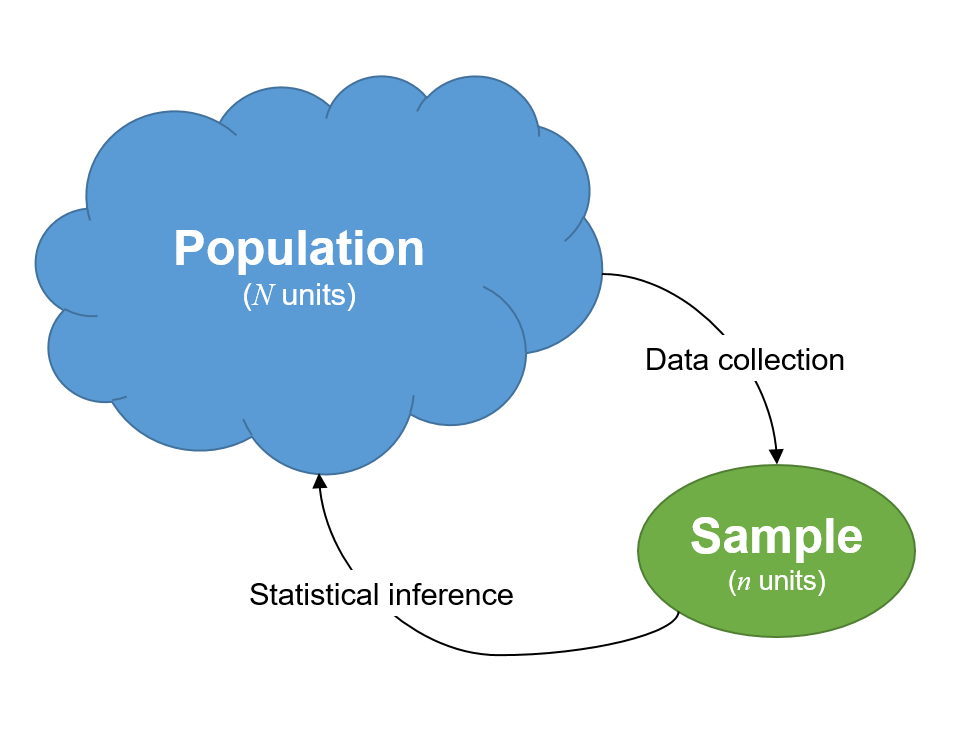
What is inference?

image source: Umberto, DAPR1

Null Hypothesis Testing

Null Hypothesis Testing

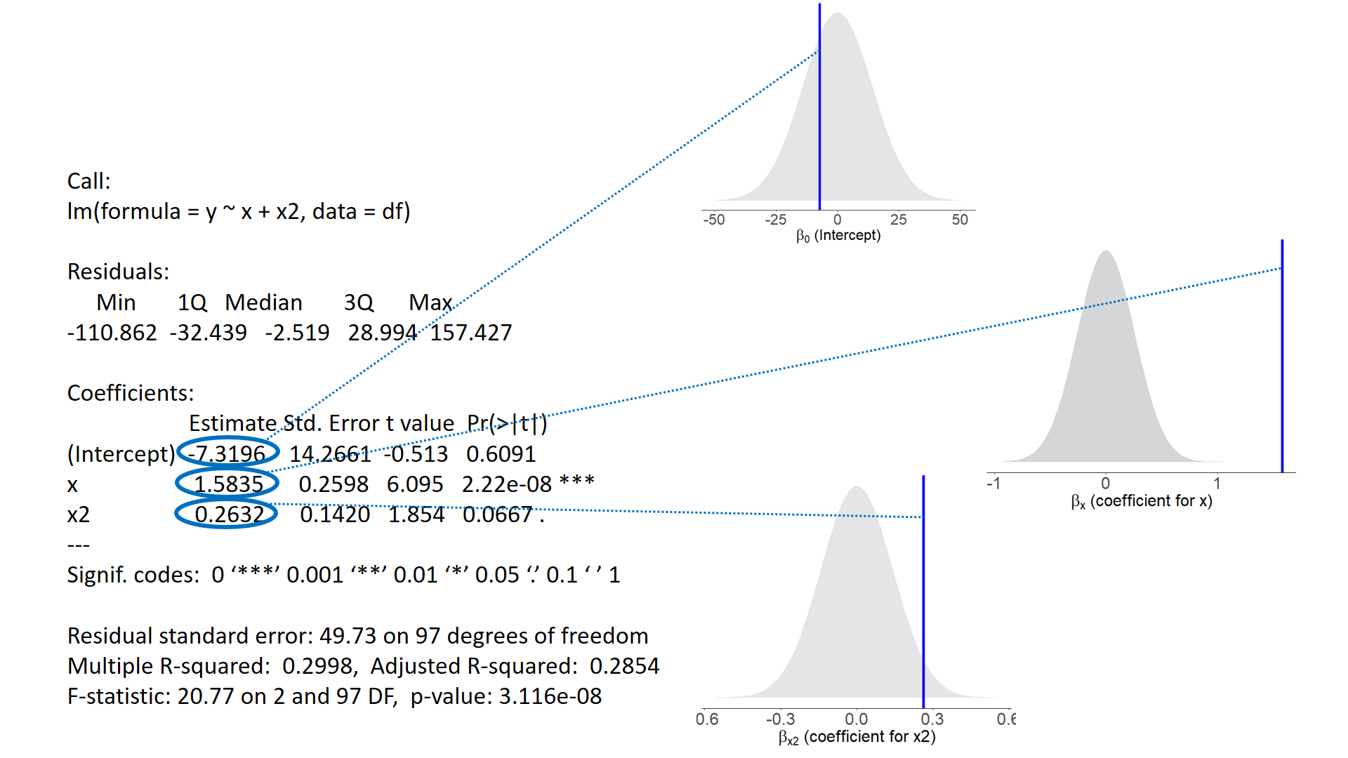
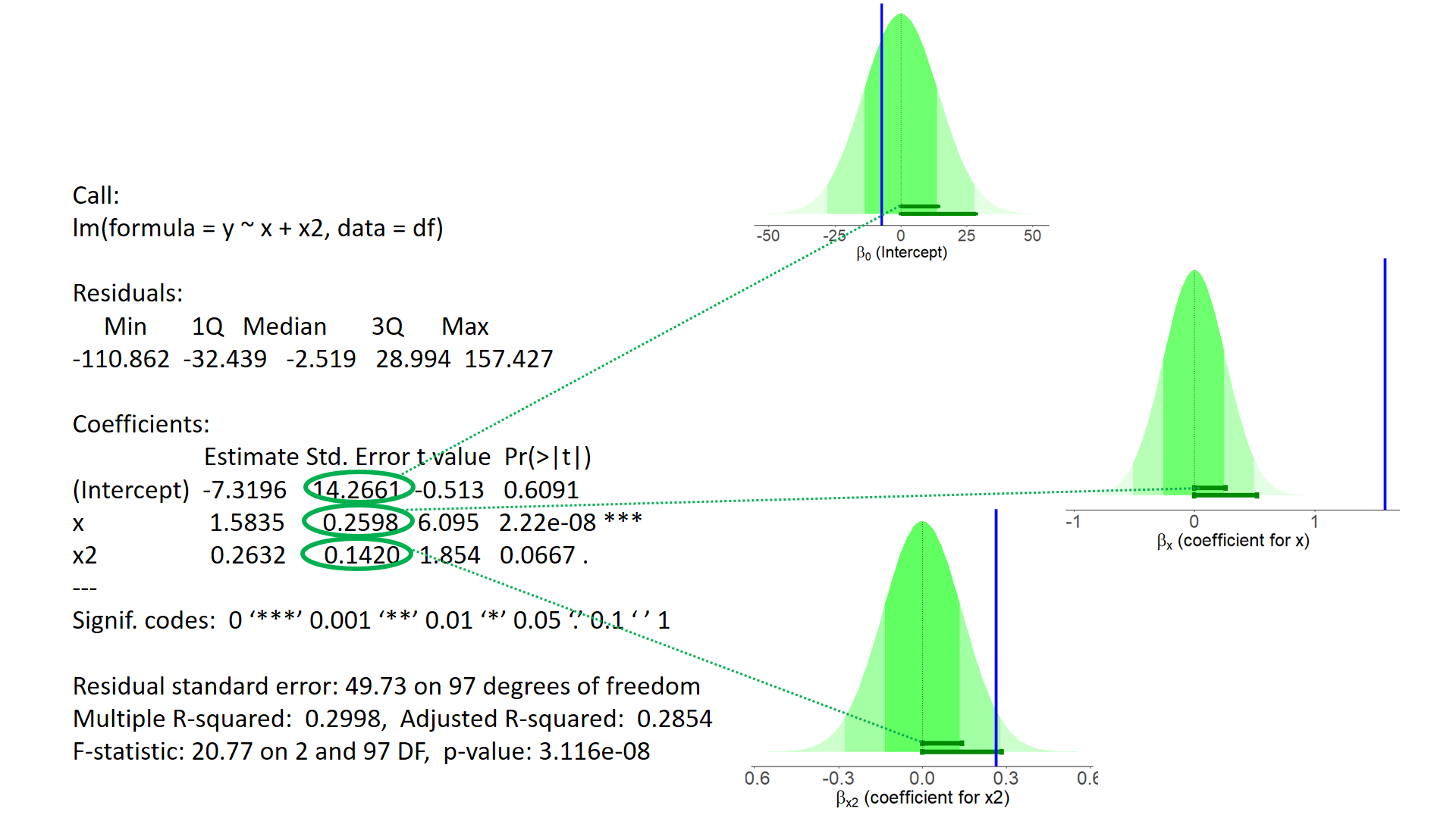
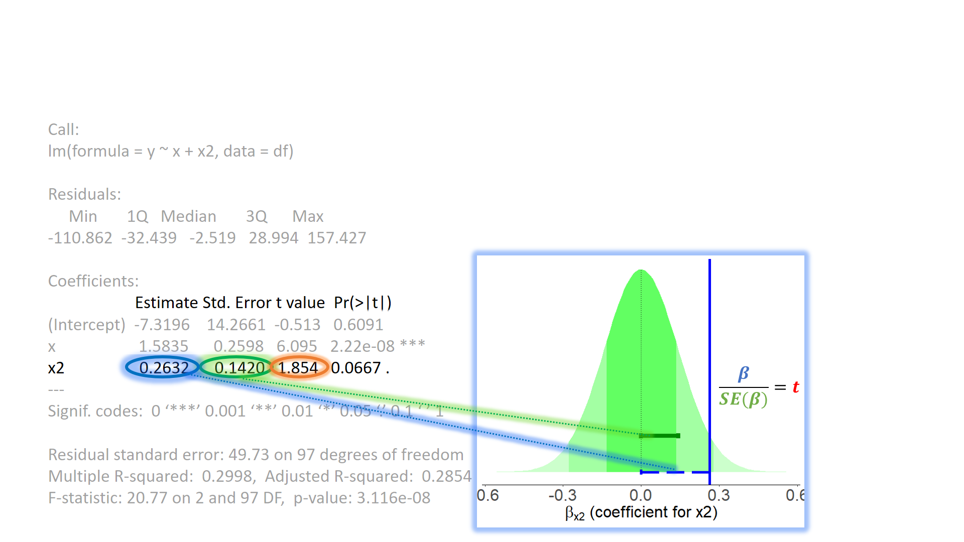
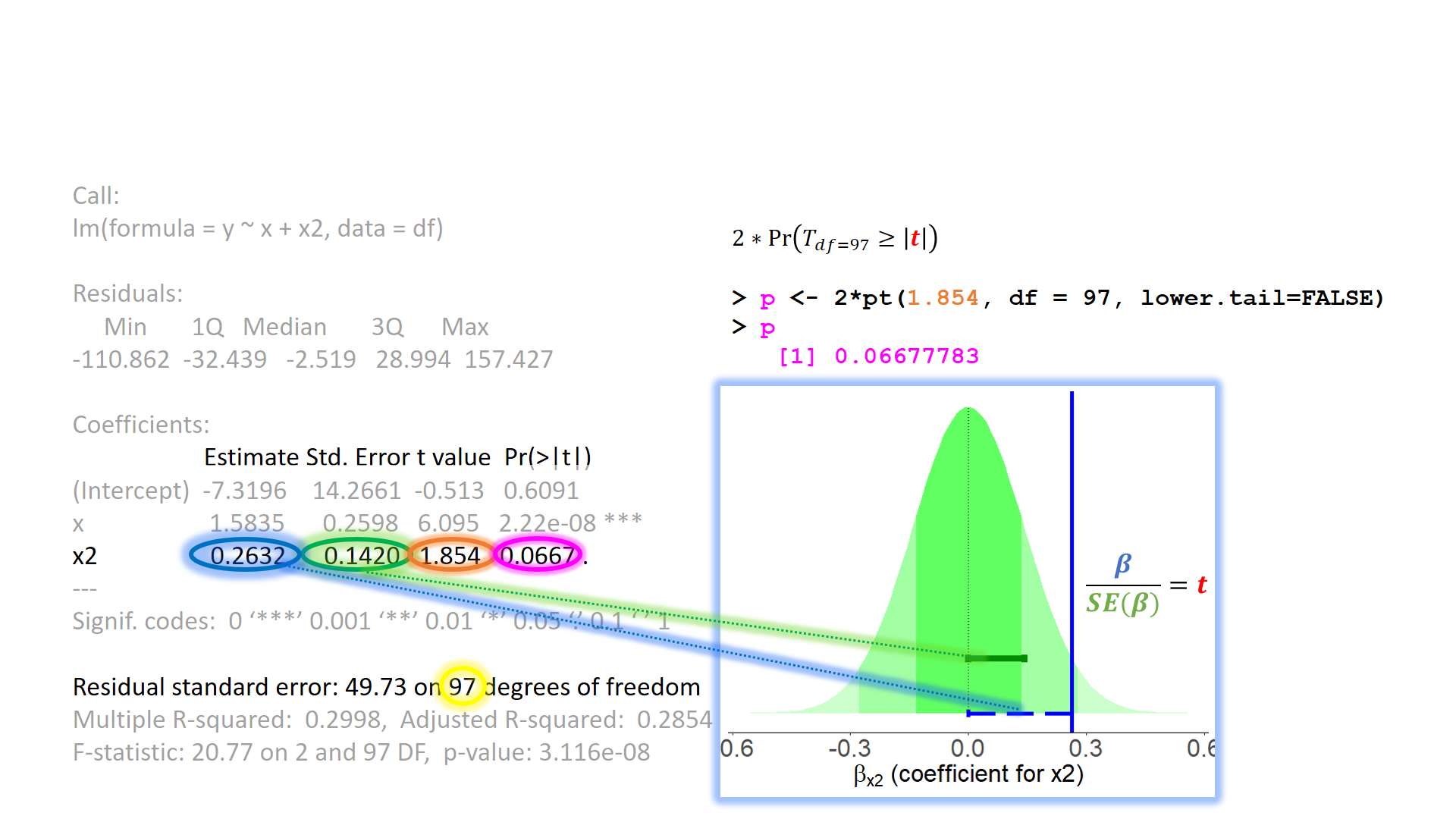
test of individual parameters

test of individual parameters (2)

test of individual parameters (3)

test of individual parameters (4)

Sums of Squares

Rather than focussing on slope coefficients, we can also think of our model in terms of sums of squares (SS).

• \(SS_{total} = \sum^{n}_{i=1}(y_i - \bar y)^2\)

• \(SS_{model} = \sum^{n}_{i=1}(\hat y_i - \bar y)^2\)

• \(SS_{residual} = \sum^{n}_{i=1}(y_i - \hat y_i)^2\)

Sums of Squares (2)

Rather than focussing on slope coefficients, we can also think of our model in terms of sums of squares (SS).

• \(SS_{total} = \sum^{n}_{i=1}(y_i - \bar y)^2\)
  • a+b+c+e
• \(SS_{model} = \sum^{n}_{i=1}(\hat y_i - \bar y)^2\)
  • a+b+c
• \(SS_{residual} = \sum^{n}_{i=1}(y_i - \hat y_i)^2\)
  • e

\(R^2\)

\(R^2 = \frac{SS_{Model}}{SS_{Total}} = 1 - \frac{SS_{Residual}}{SS_{Total}}\)

mdl <- lm(y ~ 1 + z + x)
summary(mdl)

...

Coefficients:
            Estimate Std. Error t value Pr(>|t|)   
(Intercept)   ...       ...      ...    ...
z             ...       ...      ...    ...
x             ...       ...      ...    ...
...

...
Multiple R-squared:  0.134, Adjusted R-squared:  0.116
...

tests of multiple parameters

Model comparisons:

m1 <- lm(y ~ 1 + x, data = df)

m2 <- lm(y ~ 1 + z + z2 + x, data = df)

tests of multiple parameters (2)

isolate the improvement in model fit due to inclusion of additional parameters

m1 <- lm(y ~ 1 + x, data = df)
m2 <- lm(y ~ 1 + z + z2 + x, data = df)
anova(m1,m2)

Analysis of Variance Table

Model 1: y ~ 1 + x
Model 2: y ~ 1 + z + z2 + x
  Res.Df  RSS Df Sum of Sq   F Pr(>F)    
1     98 1141                            
2     96  357  2       785 106 <2e-16 ***
---
Signif. codes:  0 '***' 0.001 '**' 0.01 '*' 0.05 '.' 0.1 ' ' 1

For linear models, model comparisons are typically testing reduction in residual sums of squares (via an \(F\) test). For models with other error distributions, we often test differences in log-likelihood (via \(\chi^2\) test).

tests of multiple parameters (3)

Test everything in the model all at once by comparing it to a ‘null model’ with no predictors:

m0 <- lm(y ~ 1, data = df)
m2 <- lm(y ~ 1 + z2 + z + x, data = df)
anova(m0,m2)

Analysis of Variance Table

Model 1: y ~ 1
Model 2: y ~ 1 + z2 + z + x
  Res.Df  RSS Df Sum of Sq    F Pr(>F)    
1     99 1232                             
2     96  357  3       875 78.6 <2e-16 ***
---
Signif. codes:  0 '***' 0.001 '**' 0.01 '*' 0.05 '.' 0.1 ' ' 1

tests of multiple parameters (4)

• Recall that a categorical predictor with \(k\) levels involves fitting \(k-1\) coefficients
• We can test “are there differences in group means?” by testing the reduction in residual sums of squares resulting from the inclusion of all \(k-1\) coefficients at once

m0 = lm(y ~ 1, data = df)
m1 = lm(y ~ 1 + species, data = df)

summary(m1)

Coefficients:
              Estimate Std. Error t value Pr(>|t|)    
(Intercept)     13.851      0.660   21.00  < 2e-16 ***
speciesdog      -3.210      0.933   -3.44  0.00086 ***
specieshorse    -3.316      0.933   -3.55  0.00059 ***
speciesparrot   -2.903      0.933   -3.11  0.00245 ** 
---
Signif. codes:  0 '***' 0.001 '**' 0.01 '*' 0.05 '.' 0.1 ' ' 1

Residual standard error: 3.3 on 96 degrees of freedom
Multiple R-squared:  0.152, Adjusted R-squared:  0.126 
F-statistic: 5.75 on 3 and 96 DF,  p-value: 0.00117

anova(m0, m1)

Analysis of Variance Table

Model 1: y ~ 1
Model 2: y ~ 1 + species
  Res.Df  RSS Df Sum of Sq    F Pr(>F)   
1     99 1232                            
2     96 1044  3       188 5.75 0.0012 **
---
Signif. codes:  0 '***' 0.001 '**' 0.01 '*' 0.05 '.' 0.1 ' ' 1

traditional ANOVA/ANCOVA

This is kind of where traditional “analysis of (co)variance” sits.

There are different ‘types’ of ANOVA..

• Type 1 (“sequential”): tests the addition of each variable entered in to the model, in order

m1 = lm(y ~ z2 + z + x, data = df)
anova(m1)

Analysis of Variance Table

Response: y
          Df Sum Sq Mean Sq F value  Pr(>F)    
z2         1    449     449   120.8 < 2e-16 ***
z          1    322     322    86.7 4.5e-15 ***
x          1    105     105    28.2 7.0e-07 ***
Residuals 96    357       4                    
---
Signif. codes:  0 '***' 0.001 '**' 0.01 '*' 0.05 '.' 0.1 ' ' 1

this is not really relevant for DAPR3, but put a pin in it here, and come back to it if your dissertation supervisor suggests that you do an ANOVA/ANCOVA. You’ve already got all the tools to do these in the regression framework with lm().

traditional ANOVA/ANCOVA

This is kind of where traditional “analysis of (co)variance” sits.

There are different ‘types’ of ANOVA..

• Type 3: tests the addition of each variable as if it were the last one entered in to the model:

m1 = lm(y ~ z2 + z + x, data = df)
car::Anova(m1, type="III")

Anova Table (Type III tests)

Response: y
            Sum Sq Df F value  Pr(>F)    
(Intercept)  12041  1  3242.2 < 2e-16 ***
z2             301  1    80.9 2.1e-14 ***
z              352  1    94.8 5.4e-16 ***
x              105  1    28.2 7.0e-07 ***
Residuals      357 96                    
---
Signif. codes:  0 '***' 0.001 '**' 0.01 '*' 0.05 '.' 0.1 ' ' 1

this is not really relevant for DAPR3, but put a pin in it here, and come back to it if your dissertation supervisor suggests that you do an ANOVA/ANCOVA. You’ve already got all the tools to do these in the regression framework with lm().

Assumptions

models have assumptions

Our model:

\(\color{red}{y} = \color{blue}{\mathbf{X \boldsymbol \beta}} + \varepsilon \qquad \text{where } \boldsymbol \varepsilon \sim N(0, \sigma) \text{ independently}\)

Our ability to generalise from the model we fit on sample data to the wider population requires making some assumptions.

• assumptions about the nature of the model (linear)

• assumptions about the nature of the errors (normal)

You can also phrase the linear model as: \(\color{red}{\boldsymbol y} \sim Normal(\color{blue}{\mathbf{X \boldsymbol \beta}}, \sigma)\)

The broader idea

All our work here is in aim of making models of the world.

• Models are models. They are simplifications. They are therefore wrong.

• Our residuals reflect everything that we don’t account for in our model. \(y - \hat{y}\)

• In an ideal world, our model accounts for all the systematic relationships. The leftovers (our residuals) are just random noise.

  • If our model is mis-specified, or we don’t measure some systematic relationship, then our residuals may reflect this.

• We check by examining how much “like randomness” the residuals appear to be (zero mean, normally distributed, constant variance, i.i.d (“independent and identically distributed”)

  • these ideas tend to get referred to as our “assumptions”

• We will never know whether our residuals contain only randomness - we can never observe everything!

assumptions

What does randomness look like?
“zero mean and constant variance”

• mean of the residuals = zero across the predicted values of the model.

• spread of residuals is normally distributed and constant across the predicted values of the model.

assumptions

What does randomness look like?
“zero mean and constant variance”

• mean of the residuals = zero across the predicted values of the model.

• spread of residuals is normally distributed and constant across the predicted values of the model.

assumptions

What does randomness look like?
“zero mean and constant variance”

• mean of the residuals = zero across the predicted values of the model.

• spread of residuals is normally distributed and constant across the predicted values of the model.

assumptions

What does randomness look like?
“zero mean and constant variance”

• mean of the residuals = zero across the predicted values of the model.

• spread of residuals is normally distributed and constant across the predicted values of the model.

plot(model)

my_model <- lm(y ~ z + x, data = df)
plot(my_model)

assumptions: the recipe book

Linearity
Independence
Normality
Equal variances

“A Line without N is a Lie!” (Umberto)

when things look weird…

first thing to do: think!

• is our model mis-specified?
  • is the relationship non-linear? higher order terms? (e.g. \(y \sim x + x^2\))
  • is there an omitted variable or interaction term?
  • given our outcome variable, do we really expect our errors to be normally distributed?

…

when things look weird…

highly skewed?

• transform the outcome variable?
  • makes things look more “normal”
  • but can make things more tricky to interpret:
    lm(y ~ x) and lm(log(y) ~ x) are quite different models

…

when things look weird…

non-constant variance?

• bootstrap*
  • do many times: resample (with replacement) your data, and refit your model.
  • obtain a distribution of parameter estimate of interest.
  • summarise the distribution to compute a confidence interval for the estimate
  • celebrate?
    
• corrected standard errors (see {lmtest} package)

…

* not great with small samples.

what about independence?

• you can’t necessarily see violations of independence in diagnostic plots - we need to think about how the data were generated.

• transformations/bootstraps/ etc don’t help us if we have violated our assumption of independence…

Group Structured Data

Examples of grouped (‘clustered’) data

• children within schools

• patients within clinics

• observations within individuals

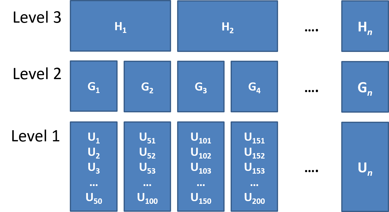
Clusters of clusters

• children within classrooms within schools within districts etc…

• patients within doctors within hospitals…

• time-periods within trials within individuals

Other relevant terms you will tend to see: “grouping structure”, “levels”, “hierarchies”.

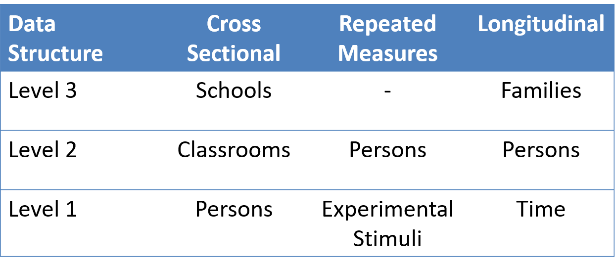
Common study designs

the impact of clustering

Measurements on observational units within a given cluster are often more similar to each other than to those in other clusters.

• For example, our measure of academic performance for children in a given class will tend to be more similar to one another (because of class specific things such as the teacher) than to children in other classes.

the impact of clustering

why?

Clustering is something systematic that our model should (arguably) take into account.

• \(\varepsilon \sim N(0, \sigma) \textbf{ independently}\)

how?

Standard errors will often be smaller than they should be, meaning that:

• confidence intervals will often be too narrow
• \(t\)-statistics will often be too large
  
• \(p\)-values will often be misleadingly small

quantifying clustering

Clustering can be expressed in terms of the expected correlation among the measurements within the same cluster - known as the intra-class correlation coefficient (ICC).

There are various formulations of ICC, but the basic principle = ratio of variance between groups to total variance.

\(\rho = \frac{\sigma^2_{b}}{\sigma^2_{b} + \sigma^2_e} \\ \qquad \\\textrm{Where:} \\ \sigma^2_{b} = \textrm{variance between clusters} \\ \sigma^2_e = \textrm{variance within clusters (residual variance)} \\\)

The larger the ICC, the lower the variability is within the clusters (relative to the variability between clusters). The greater the correlation between two observations from the same group.

Can also be interpreted as the expected correlation between two randomly drawn observations from the same group.

Working with clustered data

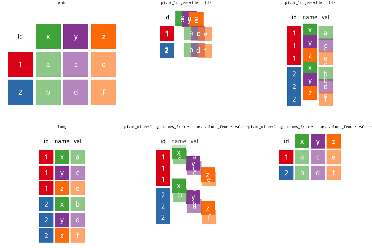
Wide Data/Long Data

Wide Data
observations are spread across columns

# A tibble: 5 × 5
  ID    age   trial_1 trial_2 trial_3
  <chr> <chr> <chr>   <chr>   <chr>  
1 001   62    10      12.5    18     
2 002   66    7.5     7       5      
3 003   22    12      14.5    11     
4 004   34    10.5    17      14     
5 ...   ...   ...     ...     ...    

Long Data
each observation of the outcome is a separate row

# A tibble: 13 × 4
   ID    age   trial   score
   <chr> <chr> <chr>   <chr>
 1 001   44    trial_1 10   
 2 001   44    trial_2 12.5 
 3 001   44    trial_3 18   
 4 002   38    trial_1 7.5  
 5 002   38    trial_2 7    
 6 002   38    trial_3 5    
 7 003   74    trial_1 12   
 8 003   74    trial_2 14.5 
 9 003   74    trial_3 11   
10 004   58    trial_1 10.5 
11 004   58    trial_2 17   
12 004   58    trial_3 14   
13 ...   ...   ...     ...  

Wide Data/Long Data

Source: Examples of wide and long representations of the same data. Source: Garrick Aden-Buie’s (\@grrrck) Tidy Animated Verbs

Long Data = plots by group

group aesthetic

ggplot(longd, aes(x=trial,y=score, group=ID))+
  geom_point(size=4)+
  geom_path()

facet_wrap()

ggplot(longd, aes(x=trial,y=score))+
  geom_point(size=4)+
  geom_path(aes(group=1))+
  facet_wrap(~ID)

Long Data = computations by-group

longd %>% 
  group_by(ID) %>%
  summarise(
    ntrials = n_distinct(trial),
    meanscore = mean(score),
    sdscore = sd(score)
  )

# A tibble: 4 × 4
  ID    ntrials meanscore sdscore
  <chr>   <int>     <dbl>   <dbl>
1 001         3      13.5    4.09
2 002         3       6.5    1.32
3 003         3      12.5    1.80
4 004         3      13.8    3.25

Modelling clustered data with lm()

Example data

Are older people more satisfied with life? 112 people from 12 different dwellings (cities/towns) in Scotland. Information on their ages and some measure of life satisfaction.

d3 <- read_csv("https://uoepsy.github.io/data/lmm_lifesatscot.csv") 
head(d3)

# A tibble: 6 × 4
    age lifesat dwelling size 
  <dbl>   <dbl> <chr>    <chr>
1    40      31 Aberdeen >100k
2    45      56 Glasgow  >100k
3    40      51 Glasgow  >100k
4    40      55 Dundee   >100k
5    40      41 Dundee   >100k
6    55      69 Perth    <100k

library(ICC)
ICCbare(x = dwelling, y = lifesat, data = d3)

[1] 0.404

Ignore it

(Complete pooling)

• lm(y ~ 1 + x, data = df)

• Information from all clusters is pooled together to estimate over x

model <- lm(lifesat ~ 1 + age, data = d3)

            Estimate Std. Error t value Pr(>|t|)    
(Intercept)   30.018      4.889    6.14  1.3e-08 ***
age            0.499      0.118    4.22  5.1e-05 ***

Ignore it

(Complete pooling)

• lm(y ~ 1 + x, data = df)

• Information from all clusters is pooled together to estimate over x

model <- lm(lifesat ~ 1 + age, data = d3)

            Estimate Std. Error t value Pr(>|t|)    
(Intercept)   30.018      4.889    6.14  1.3e-08 ***
age            0.499      0.118    4.22  5.1e-05 ***

But residuals are not independent.

Fixed Effects Models

(No pooling)

• lm(y ~ cluster + x, data = df)

• Completely partition out cluster differences in average \(y\).

• Treat every cluster as an independent entity.

model <- lm(lifesat ~ 1 + dwelling + age, data = d3)

                     Estimate Std. Error t value Pr(>|t|)    
(Intercept)           15.3330     4.1493    3.70  0.00036 ***
dwellingDumfries       8.0741     3.8483    2.10  0.03844 *  
dwellingDundee        15.9882     3.8236    4.18  6.3e-05 ***
dwellingDunfermline   26.2600     3.8910    6.75  1.0e-09 ***
dwellingEdinburgh     12.6929     3.8195    3.32  0.00125 ** 
dwellingFort William   1.3577     3.8999    0.35  0.72849    
dwellingGlasgow       18.2906     3.8213    4.79  5.9e-06 ***
dwellingInverness      5.0718     3.8542    1.32  0.19124    
...  ...
...  ...

age                    0.6047     0.0888    6.81  7.6e-10 ***
---

Fixed Effects Models

(No pooling)

• lm(y ~ cluster * x, data = df)

• Completely partition out cluster differences in \(y \sim x\).

• Treat every cluster as an independent entity.

model <- lm(lifesat ~ 1 + dwelling * age, data = d3)

Coefficients:
                         Estimate Std. Error t value  Pr(>|t|)    
(Intercept)                -4.345      8.867   -0.49   0.62532    
dwellingDumfries           13.480     14.370    0.94   0.35078    
dwellingDundee             59.479     17.650    3.37   0.00112 ** 
dwellingDunfermline        42.938     17.206    2.50   0.01444 *  
...  ...

age                         1.159      0.239    4.84 0.0000054 ***
dwellingDumfries:age       -0.206      0.360   -0.57   0.56813    
dwellingDundee:age         -1.181      0.463   -2.55   0.01243 *  
dwellingDunfermline:age    -0.486      0.408   -1.19   0.23638    
...  ...

It doesn’t matter if 99/100 clusters all show one pattern, we’re happy to let cluster 100 do it’s own thing.

Fixed Effects Models

(No pooling)

• lm(y ~ cluster * x, data = df)

• Completely partition out cluster differences in \(y \sim x\).

• Treat every cluster as an independent entity.

• Prevents us from studying cluster level effects.

model <- lm(lifesat ~ 1 + dwelling * age + size, data = d3)

Coefficients: (1 not defined because of singularities)
                         Estimate Std. Error t value  Pr(>|t|)    
(Intercept)                -4.345      8.867   -0.49   0.62532    
dwellingDumfries           13.480     14.370    0.94   0.35078    
dwellingDundee             59.479     17.650    3.37   0.00112 ** 
dwellingDunfermline        42.938     17.206    2.50   0.01444 *  
...  ...
...  ...

dwellingPaisley            28.665     16.732    1.71   0.09020 .  
dwellingPerth              27.473     12.901    2.13   0.03600 *  
dwellingStirling           42.272     13.379    3.16   0.00217 ** 
age                         1.159      0.239    4.84 0.0000054 ***
size>100k                      NA         NA      NA        NA    
dwellingDumfries:age       -0.206      0.360   -0.57   0.56813    
dwellingDundee:age         -1.181      0.463   -2.55   0.01243 *  
... ...

              size
dwelling       <100k >100k
  Aberdeen         0    10
  Dumfries        10     0
  Dundee           0    10
  Dunfermline     10     0
  Edinburgh        0    10
  Fort William    10     0
  Glasgow          0    10
  Inverness       10     0
  Kirkcaldy        2     0
  Paisley         10     0
  Perth           10     0
  Stirling        10     0

Summary

• we can fit a linear regression model which takes the form \(\color{red}{y} = \color{blue}{\mathbf{X} \boldsymbol{\beta}} + \boldsymbol{\varepsilon}\)

• in R, we fit this with lm(y ~ x1 + .... xk, data = mydata).

• we can extend this to different link functions to model outcome variables which follow different distributions.

• when drawing inferences from a fitted model to the broader population, we rely on certain assumptions.

  • one of these is that the errors are independent.

This week

Tasks

Complete readings

Attend your lab and work together on the exercises

Complete the weekly quiz

Support

Piazza forum!

Office hours (see Learn page for details)