class: center, middle, inverse, title-slide # <b>Centering Predictors<br>Generalisations</b> ## Data Analysis for Psychology in R 3 ### Josiah King, Umberto Noè, Tom Booth ### Department of Psychology<br/>The University of Edinburgh ### AY 2021-2022 --- class: inverse, center, middle <h2>Part 1: Centering Predictors</h2> <h2 style="text-align: left;opacity:0.3;">Part 2: GLMM</h2> --- # Centering .pull-left[ Suppose we have a variable for which the mean is 100. <!-- --> ] -- .pull-right[ We can re-center this so that the mean becomes zero: <!-- --> ] --- count:false # Centering .pull-left[ Suppose we have a variable for which the mean is 100. <!-- --> ] .pull-right[ We can re-center this so that _any_ value becomes zero: <!-- --> ] --- # Scaling .pull-left[ Suppose we have a variable for which the mean is 100. The standard deviation is 15 <!-- --> ] -- .pull-right[ We can scale this so that a change in 1 is equivalent to a change in 1 standard deviation: <!-- --> ] --- # Centering predictors in LM .pull-left[ ```r m1 <- lm(y~x,data=df) m2 <- lm(y~scale(x, center=T,scale=F),data=df) m3 <- lm(y~scale(x, center=T,scale=T),data=df) m4 <- lm(y~I(x-5), data=df) ``` ] --- count:false # Centering predictors in LM .pull-left[ ```r m1 <- lm(y~x,data=df) m2 <- lm(y~scale(x, center=T,scale=F),data=df) m3 <- lm(y~scale(x, center=T,scale=T),data=df) m4 <- lm(y~I(x-5), data=df) ``` ```r anova(m1,m2,m3,m4) ``` ``` ## Analysis of Variance Table ## ## Model 1: y ~ x ## Model 2: y ~ scale(x, center = T, scale = F) ## Model 3: y ~ scale(x, center = T, scale = T) ## Model 4: y ~ I(x - 5) ## Res.Df RSS Df Sum of Sq F Pr(>F) ## 1 198 177 ## 2 198 177 0 0 ## 3 198 177 0 0 ## 4 198 177 0 0 ``` ] -- .pull-right[ <img src="04_centeringglmer_files/figure-html/unnamed-chunk-11-1.png" style="display: block; margin: auto;" /> ] --- # Big Fish Little Fish <img src="04_centeringglmer_files/figure-html/unnamed-chunk-13-1.png" style="display: block; margin: auto;" /> data available at https://uoepsy.github.io/data/bflp.csv --- # Things are different with multi-level data <img src="04_centeringglmer_files/figure-html/unnamed-chunk-14-1.png" style="display: block; margin: auto;" /> --- # Multiple means .pull-left[ __Grand mean__ 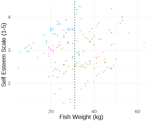<!-- --> ] -- .pull-right[ __Group means__ 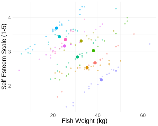<!-- --> ] --- # Group mean centering .pull-left[ <center>__ `\(x_{ij} - \bar{x}_i\)` __</center> 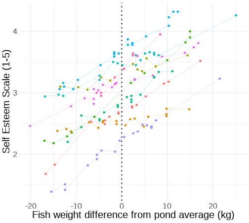<!-- --> ] --- # Group-mean centering <br> <img src="jk_img_sandbox/center.gif" style="display: block; margin: auto;" /> --- # Group mean centering .pull-left[ <center>__ `\(x_{ij} - \bar{x}_i\)` __</center> <!-- --> ] .pull-right[ <center>__ `\(\bar{x}_i\)` __</center> 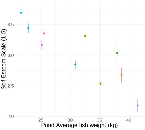<!-- --> ] --- # Disaggregating within & between .pull-left[ **RE model** $$ `\begin{align} y_{ij} &= \beta_{0i} + \beta_{1}(x_j) + \varepsilon_{ij} \\ \beta_{0i} &= \gamma_{00} + \zeta_{0i} \\ ... \\ \end{align}` $$ ```r rem <- lmer(self_esteem ~ fish_weight + (1 | pond), data=bflp) ``` ] -- .pull-right[ **Within-between model** $$ `\begin{align} y_{ij} &= \beta_{0i} + \beta_{1}(\bar{x}_i) + \beta_2(x_{ij} - \bar{x}_i)+ \varepsilon_{ij} \\ \beta_{0i} &= \gamma_{00} + \zeta_{0i} \\ ... \\ \end{align}` $$ ```r bflp <- bflp %>% group_by(pond) %>% mutate( fw_pondm = mean(fish_weight), fw_pondc = fish_weight - mean(fish_weight) ) %>% ungroup wbm <- lmer(self_esteem ~ fw_pondm + fw_pondc + (1 | pond), data=bflp) fixef(wbm) ``` ``` ## (Intercept) fw_pondm fw_pondc ## 4.76802 -0.05586 0.04067 ``` ] --- # Disaggregating within & between .pull-left[ <img src="04_centeringglmer_files/figure-html/unnamed-chunk-25-1.png" style="display: block; margin: auto;" /> ] .pull-right[ **Within-between model** $$ `\begin{align} y_{ij} &= \beta_{0i} + \beta_{1}(\bar{x}_i) + \beta_2(x_{ij} - \bar{x}_i)+ \varepsilon_{ij} \\ \beta_{0i} &= \gamma_{00} + \zeta_{0i} \\ ... \\ \end{align}` $$ ```r bflp <- bflp %>% group_by(pond) %>% mutate( fw_pondm = mean(fish_weight), fw_pondc = fish_weight - mean(fish_weight) ) %>% ungroup wbm <- lmer(self_esteem ~ fw_pondm + fw_pondc + (1 | pond), data=bflp) fixef(wbm) ``` ``` ## (Intercept) fw_pondm fw_pondc ## 4.76802 -0.05586 0.04067 ``` ] --- # A more realistic example .pull-left[ A research study investigates how anxiety is associated with drinking habits. Data was collected from 50 participants. Researchers administered the generalised anxiety disorder (GAD-7) questionnaire to measure levels of anxiety over the past week, and collected information on the units of alcohol participants had consumed within the week. Each participant was observed on 10 different occasions. ] .pull-right[ <!-- --> data available at https://uoepsy.github.io/data/alcgad.csv ] --- # A more realistic example .pull-left[ Is being more nervous (than you usually are) associated with higher consumption of alcohol? ] .pull-right[ <!-- --> ] --- # A more realistic example .pull-left[ Is being generally more nervous (relative to others) associated with higher consumption of alcohol? ] .pull-right[ <!-- --> ] --- # Modelling within & between effects .pull-left[ ```r alcgad <- alcgad %>% group_by(ppt) %>% mutate( gadm=mean(gad), gadmc=gad-gadm ) alcmod <- lmer(alcunits ~ gadm + gadmc + (1 + gadmc | ppt), data=alcgad, control=lmerControl(optimizer = "bobyqa")) ``` ] .pull-right[ ```r summary(alcmod) ``` ``` ## Linear mixed model fit by REML ['lmerMod'] ## Formula: alcunits ~ gadm + gadmc + (1 + gadmc | ppt) ## Data: alcgad ## Control: lmerControl(optimizer = "bobyqa") ## ## REML criterion at convergence: 1424 ## ## Scaled residuals: ## Min 1Q Median 3Q Max ## -2.8466 -0.6264 0.0642 0.6292 3.0281 ## ## Random effects: ## Groups Name Variance Std.Dev. Corr ## ppt (Intercept) 3.7803 1.944 ## gadmc 0.0935 0.306 -0.30 ## Residual 1.7234 1.313 ## Number of obs: 375, groups: ppt, 50 ## ## Fixed effects: ## Estimate Std. Error t value ## (Intercept) 14.5802 0.8641 16.87 ## gadm -0.7584 0.1031 -7.35 ## gadmc 0.6378 0.0955 6.68 ## ## Correlation of Fixed Effects: ## (Intr) gadm ## gadm -0.945 ## gadmc -0.055 0.012 ``` ] --- # Modelling within & between interactions .pull-left[ ```r alcmod <- lmer(alcunits ~ (gadm + gadmc)*interv + (1 | ppt), data=alcgad, control=lmerControl(optimizer = "bobyqa")) ``` ] .pull-right[ ```r summary(alcmod) ``` ``` ## Linear mixed model fit by REML ['lmerMod'] ## Formula: alcunits ~ (gadm + gadmc) * interv + (1 | ppt) ## Data: alcgad ## Control: lmerControl(optimizer = "bobyqa") ## ## REML criterion at convergence: 1404 ## ## Scaled residuals: ## Min 1Q Median 3Q Max ## -2.8183 -0.6354 0.0142 0.5928 3.0874 ## ## Random effects: ## Groups Name Variance Std.Dev. ## ppt (Intercept) 3.59 1.9 ## Residual 1.69 1.3 ## Number of obs: 375, groups: ppt, 50 ## ## Fixed effects: ## Estimate Std. Error t value ## (Intercept) 14.858 1.275 11.65 ## gadm -0.876 0.154 -5.70 ## gadmc 1.092 0.128 8.56 ## interv -0.549 1.711 -0.32 ## gadm:interv 0.205 0.205 1.00 ## gadmc:interv -0.757 0.166 -4.57 ## ## Correlation of Fixed Effects: ## (Intr) gadm gadmc interv gdm:nt ## gadm -0.939 ## gadmc 0.000 0.000 ## interv -0.746 0.700 0.000 ## gadm:interv 0.705 -0.750 0.000 -0.944 ## gadmc:intrv 0.000 0.000 -0.770 0.000 0.000 ``` ] --- # The total effect .pull-left[ ```r alcmod2 <- lmer(alcunits ~ gad + (1 | ppt), data=alcgad, control=lmerControl(optimizer = "bobyqa")) ``` ] .pull-right[ ```r summary(alcmod2) ``` ``` ## Linear mixed model fit by REML ['lmerMod'] ## Formula: alcunits ~ gad + (1 | ppt) ## Data: alcgad ## Control: lmerControl(optimizer = "bobyqa") ## ## REML criterion at convergence: 1494 ## ## Scaled residuals: ## Min 1Q Median 3Q Max ## -2.9940 -0.6414 0.0258 0.5808 2.9825 ## ## Random effects: ## Groups Name Variance Std.Dev. ## ppt (Intercept) 14.32 3.78 ## Residual 1.83 1.35 ## Number of obs: 375, groups: ppt, 50 ## ## Fixed effects: ## Estimate Std. Error t value ## (Intercept) 5.1787 0.8198 6.32 ## gad 0.4281 0.0779 5.50 ## ## Correlation of Fixed Effects: ## (Intr) ## gad -0.752 ``` ] --- # Within & Between .pull-left[ <!-- --> ] .pull-right[ <!-- --> ] --- count:false # Within & Between .pull-left[ <!-- --> ] -- .pull-right[ <!-- --> ] --- # Summary - Applying the same linear transformation to a predictor (e.g. grand-mean centering, or standardising) makes __no difference__ to our model or significance tests - but it may change the meaning and/or interpretation of our parameters - When data are clustered, we can apply group-level transformations, e.g. __group-mean centering.__ - Group-mean centering our predictors allows us to disaggregate __within__ from __between__ effects. - allowing us to ask the theoretical questions that we are actually interested in --- class: inverse, center, middle, animated, rotateInDownLeft # End of Part 1 --- class: inverse, center, middle <h2 style="text-align: left;opacity:0.3;">Part 1: Centering Predictors</h2> <h2>Part 2: GLMM</h2> --- # lm() and glm() .pull-left[ ### lm() $$ `\begin{align} & \color{red}{y} = \color{blue}{\beta_0 + \beta_1(x_1) + ... + \beta_k(x_k)} + \mathbf{\boldsymbol{\varepsilon}}\\ \end{align}` $$ ] --- count:false # lm() and glm() .pull-left[ ### lm() $$ `\begin{align} & \color{red}{y} = \color{blue}{\underbrace{\beta_0 + \beta_1(x_1) + ... + \beta_k(x_k)}_{\mathbf{X \boldsymbol{\beta}}}} + \boldsymbol{\varepsilon} \\ \end{align}` $$ ] --- count:false # lm() and glm() .pull-left[ ### lm() $$ `\begin{align} & \color{red}{y} = \color{blue}{\underbrace{\beta_0 + \beta_1(x_1) + ... + \beta_k(x_k)}_{\mathbf{X \boldsymbol{\beta}}}} + \boldsymbol{\varepsilon} \\ & \text{where } -\infty \leq \color{red}{y} \leq \infty \\ \end{align}` $$ ] -- .pull-right[ ### &nbsp; $$ `\begin{align} \color{red}{??} = & \color{blue}{\underbrace{\beta_0 + \beta_1(x_1) + ... + \beta_k(x_k)}_{\mathbf{X \boldsymbol{\beta}}}} + \boldsymbol{\varepsilon} \\ \end{align}` $$ ] --- count:false # lm() and glm() .pull-left[ ### lm() $$ `\begin{align} & \color{red}{y} = \color{blue}{\underbrace{\beta_0 + \beta_1(x_1) + ... + \beta_k(x_k)}_{\mathbf{X \boldsymbol{\beta}}}} + \boldsymbol{\varepsilon} \\ & \text{where } -\infty \leq \color{red}{y} \leq \infty \\ \end{align}` $$ ] .pull-right[ ### glm() $$ `\begin{align} \color{red}{ln \left( \frac{p}{1-p} \right) } & = \color{blue}{\underbrace{\beta_0 + \beta_1(x_1) + ... + \beta_k(x_k)}_{\mathbf{X \boldsymbol{\beta}}}} + \boldsymbol{\varepsilon} \\ & \text{where } 0 \leq p \leq 1 \\ \end{align}` $$ ] --- count:false # lm() and glm() .pull-left[ ### lm() $$ `\begin{align} & \color{red}{y} = \color{blue}{\underbrace{\beta_0 + \beta_1(x_1) + ... + \beta_k(x_k)}_{\mathbf{X \boldsymbol{\beta}}}} + \boldsymbol{\varepsilon} \\ & \text{where } -\infty \leq \color{red}{y} \leq \infty \\ \end{align}` $$ ] .pull-right[ ### glm() $$ `\begin{align} \color{red}{ln \left( \frac{p}{1-p} \right) } & = \color{blue}{\underbrace{\beta_0 + \beta_1(x_1) + ... + \beta_k(x_k)}_{\mathbf{X \boldsymbol{\beta}}}} + \boldsymbol{\varepsilon} \\ & \text{where } 0 \leq p \leq 1 \\ \end{align}` $$ glm() is the __generalised__ linear model. we can specify the link function to model outcomes with different distributions. this allows us to fit models such as the _logistic_ regression model: ```{} glm(y~x, family = binomial(link="logit")) ``` ] --- # logistic regression visualised .pull-left[ ### continuous outcome <br><br> <!-- --> ] .pull-right[ ### binary outcome <br><br> 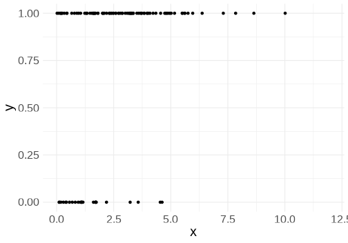<!-- --> ] --- count:false # logistic regression visualised .pull-left[ ### linear regression we model __y__ directly as linear combination of one or more predictor variables 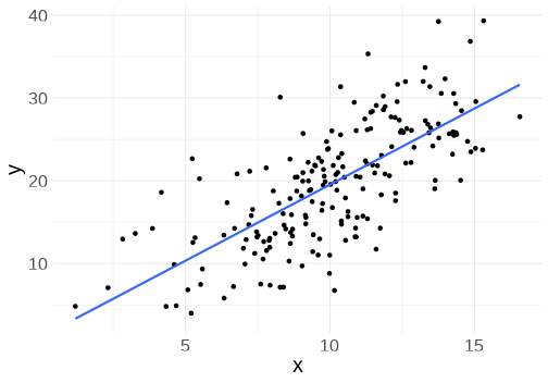<!-- --> ] .pull-right[ ### logistic regression __probability__ is _not_ linear.. but we can model it indirectly 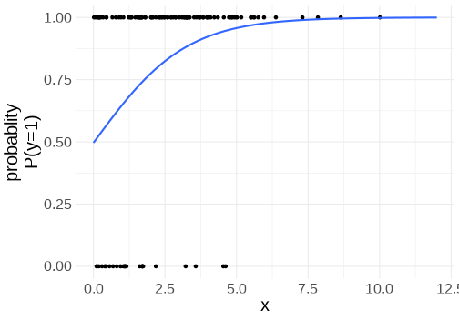<!-- --> ] --- count:false # logistic regression visualised `\(ln \left( \frac{p}{1-p} \right)\)` __log-odds__ are linear <img src="jk_img_sandbox/logoddp.png" width="1977" height="400px" /> --- # lmer() and glmer() .pull-left[ 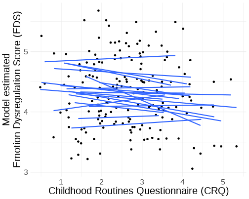<!-- --> ] .pull-right[ <!-- --> ] --- count:false # lmer() and glmer() .pull-left[ <!-- --> ] .pull-right[ <!-- --> ] --- # fitting a glmer() .pull-left[ > Researchers are interested in whether the level of routine a child has in daily life influences their probability of receiving a detention at school. 200 pupils from 20 schools completed a survey containing the Child Routines Questionnaire (CRQ), and a binary variable indicating whether or not they had received detention in the past school year. ```r crq <- read_csv("https://uoepsy.github.io/data/crqdetentiondata.csv") head(crq) ``` ``` ## # A tibble: 6 × 7 ## emot_dysreg crq int schoolid sleep age detention ## <dbl> <dbl> <chr> <chr> <chr> <dbl> <dbl> ## 1 4.12 1.92 Treatment school1 <8hr 14 1 ## 2 3.22 1.65 Treatment school1 <8hr 11 1 ## 3 4.86 3.56 Treatment school1 <8hr 16 1 ## 4 4.79 1.45 Treatment school1 8hr+ 16 1 ## 5 3.58 0.81 Treatment school1 <8hr 12 1 ## 6 4.41 2.71 Treatment school1 <8hr 15 0 ``` ] .pull-right[ ```r detentionmod <- glmer(detention ~ crq + (1 + crq | schoolid), data = crq, family="binomial") summary(detentionmod) ``` ``` ## Generalized linear mixed model fit by maximum likelihood (Laplace ## Approximation) [glmerMod] ## Family: binomial ( logit ) ## Formula: detention ~ crq + (1 + crq | schoolid) ## Data: crq ## ## AIC BIC logLik deviance df.resid ## 180.0 195.8 -85.0 170.0 169 ## ## Scaled residuals: ## Min 1Q Median 3Q Max ## -2.419 -0.450 0.119 0.504 1.826 ## ## Random effects: ## Groups Name Variance Std.Dev. Corr ## schoolid (Intercept) 2.577 1.605 ## crq 0.414 0.643 -0.52 ## Number of obs: 174, groups: schoolid, 20 ## ## Fixed effects: ## Estimate Std. Error z value Pr(>|z|) ## (Intercept) 5.472 1.184 4.62 0.0000038 *** ## crq -2.126 0.465 -4.57 0.0000049 *** ## --- ## Signif. codes: 0 '***' 0.001 '**' 0.01 '*' 0.05 '.' 0.1 ' ' 1 ## ## Correlation of Fixed Effects: ## (Intr) ## crq -0.929 ``` ] --- # fitting a glmer() .pull-left[ > Researchers are interested in whether the level of routine a child has in daily life influences their probability of receiving a detention at school. 200 pupils from 20 schools completed a survey containing the Child Routines Questionnaire (CRQ), and a binary variable indicating whether or not they had received detention in the past school year. ```r crq <- read_csv("https://uoepsy.github.io/data/crqdetentiondata.csv") head(crq) ``` ``` ## # A tibble: 6 × 7 ## emot_dysreg crq int schoolid sleep age detention ## <dbl> <dbl> <chr> <chr> <chr> <dbl> <dbl> ## 1 4.12 1.92 Treatment school1 <8hr 14 1 ## 2 3.22 1.65 Treatment school1 <8hr 11 1 ## 3 4.86 3.56 Treatment school1 <8hr 16 1 ## 4 4.79 1.45 Treatment school1 8hr+ 16 1 ## 5 3.58 0.81 Treatment school1 <8hr 12 1 ## 6 4.41 2.71 Treatment school1 <8hr 15 0 ``` ] .pull-right[ ```r detentionmod <- glmer(detention ~ crq + (1 + crq | schoolid), data = crq, family="binomial") exp(fixef(detentionmod)) ``` ``` ## (Intercept) crq ## 237.8341 0.1193 ``` ] --- # interpretating coefficients - `lm(y ~ x + ...)` - `\(\beta_x\)` denotes the change in the average `\(y\)` when `\(x\)` is increased by one unit and all other covariates are fixed. - `lmer(y ~ x + ... + (1 + x + ... | cluster))` - `\(\beta_x\)` denotes the change in the average `\(y\)` when `\(x\)` is increased by one unit, averaged across clusters - `glmer(ybin ~ x + ... + (1 + x + ... | cluster), family=binomial)` - `\(e^{\beta_x}\)` denotes the change in the average `\(y\)` when `\(x\)` is increased by one unit, __holding cluster constant.__ --- class: extra exclude: FALSE # why are glmer() coefficients cluster-specific? consider a __linear__ multilevel model: `lmer(respiratory_rate ~ treatment + (1|hospital))` Imagine two patients from different hospitals. One is has a treatment, one does not. - patient `\(j\)` from hospital `\(i\)` is "control" - patient `\(j'\)` from hospital `\(i'\)` is "treatment" The difference in estimated outcome between patient `\(j\)` and patient `\(j'\)` is the "the effect of having treatment" plus the distance in random deviations between hospitals `\(i\)` and `\(i'\)` model for patient `\(j\)` from hospital `\(i\)` `\(\hat{y}_{ij} = (\gamma_{00} + \zeta_{0i}) + \beta_1 (Treatment_{ij} = 0)\)` model for patient `\(j'\)` from hospital `\(i'\)` `\(\hat{y}_{i'j'} = (\gamma_{00} + \zeta_{0i'}) + \beta_1 (Treatment_{i'j'} = 1)\)` difference: `\(\hat{y}_{i'j'} - \hat{y}_{ij} = \beta_1 + (\zeta_{0i'} - \zeta_{0i}) = \beta_1\)` Because `\(\zeta \sim N(0,\sigma_\zeta)\)`, the differences between all different `\(\zeta_{0i'} - \zeta_{0i}\)` average out to be 0. ??? the zeta differences here will be, on average 0. hist(replicate(1000, mean(map_dbl(combn(rnorm(100),2, simplify=F), diff))),breaks=20) --- class: extra exclude: FALSE # why are glmer() coefficients cluster-specific? consider a __logistic__ multilevel model: `glmer(needs_op ~ treatment + (1|hospital), family="binomial")` Imagine two patients from different hospitals. One is has a treatment, one does not. - patient `\(j\)` from hospital `\(i\)` is "control" - patient `\(j'\)` from hospital `\(i'\)` is "treatment" The difference in __probability of outcome__ between patient `\(j\)` and patient `\(j'\)` is the "the effect of having treatment" plus the distance in random deviations between hospitals `\(i\)` and `\(i'\)` model for patient `\(j\)` from hospital `\(i\)` `\(log \left( \frac{p_{ij}}{1 - p_{ij}} \right) = (\gamma_{00} + \zeta_{0i}) + \beta_1 (Treatment_{ij} = 0)\)` model for patient `\(j'\)` from hospital `\(i'\)` `\(log \left( \frac{p_{i'j'}}{1 - p_{i'j'}} \right) = (\gamma_{00} + \zeta_{0i'}) + \beta_1 (Treatment_{i'j'} = 1)\)` difference (log odds): `\(log \left( \frac{p_{i'j'}}{1 - p_{i'j'}} \right) - log \left( \frac{p_{ij}}{1 - p_{ij}} \right) = \beta_1 + (\zeta_{0i'} - \zeta_{0i})\)` --- class: extra exclude: FALSE # why are glmer() coefficients cluster-specific? consider a __logistic__ multilevel model: `glmer(needs_op ~ treatment + (1|hospital), family="binomial")` Imagine two patients from different hospitals. One is has a treatment, one does not. - patient `\(j\)` from hospital `\(i\)` is "control" - patient `\(j'\)` from hospital `\(i'\)` is "treatment" The difference in __probability of outcome__ between patient `\(j\)` and patient `\(j'\)` is the "the effect of having treatment" plus the distance in random deviations between hospitals `\(i\)` and `\(i'\)` model for patient `\(j\)` from hospital `\(i\)` `\(log \left( \frac{p_{ij}}{1 - p_{ij}} \right) = (\gamma_{00} + \zeta_{0i}) + \beta_1 (Treatment_{ij} = 0)\)` model for patient `\(j'\)` from hospital `\(i'\)` `\(log \left( \frac{p_{i'j'}}{1 - p_{i'j'}} \right) = (\gamma_{00} + \zeta_{0i'}) + \beta_1 (Treatment_{i'j'} = 1)\)` difference (odds ratio): `\(\frac{p_{i'j'}/(1 - p_{i'j'})}{p_{ij}/(1 - p_{ij})} = \exp(\beta_1 + (\zeta_{0i'} - \zeta_{0i}))\)` --- class: extra exclude: FALSE # why are glmer() coefficients cluster-specific? consider a __logistic__ multilevel model: `glmer(needs_op ~ treatment + (1|hospital), family="binomial")` Imagine two patients from different hospitals. One is has a treatment, one does not. - patient `\(j\)` from hospital `\(i\)` is "control" - patient `\(j'\)` from hospital `\(i'\)` is "treatment" The difference in __probability of outcome__ between patient `\(j\)` and patient `\(j'\)` is the "the effect of having treatment" plus the distance in random deviations between hospitals `\(i\)` and `\(i'\)` model for patient `\(j\)` from hospital `\(i\)` `\(log \left( \frac{p_{ij}}{1 - p_{ij}} \right) = (\gamma_{00} + \zeta_{0i}) + \beta_1 (Treatment_{ij} = 0)\)` model for patient `\(j'\)` from hospital `\(i'\)` `\(log \left( \frac{p_{i'j'}}{1 - p_{i'j'}} \right) = (\gamma_{00} + \zeta_{0i'}) + \beta_1 (Treatment_{i'j'} = 1)\)` difference (odds ratio): `\(\frac{p_{i'j'}/(1 - p_{i'j'})}{p_{ij}/(1 - p_{ij})} = \exp(\beta_1 + (\zeta_{0i'} - \zeta_{0i})) \neq \exp(\beta_1)\)` --- class: extra exclude: FALSE # why are glmer() coefficients cluster-specific? consider a __logistic__ multilevel model: `glmer(needs_op ~ treatment + (1|hospital), family="binomial")` Hence, the interpretation of `\(e^{\beta_1}\)` is not the odds ratio for the effect of treatment "averaged over hospitals", but rather for patients _from the same hospital_. --- # Summary - Differences between linear and logistic multi-level models are analogous to the differences between single-level linear and logistic regression models. - Fixed effects in logistic multilevel models are "conditional upon" holding the cluster constant. --- class: inverse, center, middle, animated, rotateInDownLeft # End