class: center, middle, inverse, title-slide # <b>Assumptions & Diagnostics<br>More random effects</b> ## Data Analysis for Psychology in R 3 ### Josiah King, Umberto Noè, Tom Booth ### Department of Psychology<br/>The University of Edinburgh ### AY 2021-2022 --- class: inverse, center, middle <h2>Part 1: Assumptions</h2> <h2 style="text-align: left;opacity:0.3;">Part 2: Case Diagnostics in MLM</h2> <h2 style="text-align: left;opacity:0.3;">Part 3: Random Effect Structures</h2> --- # Assumptions in LM .pull-left[ #### The general idea - `\(\varepsilon_i \sim N(0,\sigma^2)\)` iid - "zero mean and constant variance" 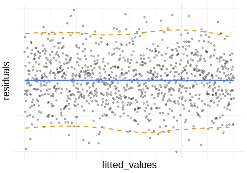<!-- --> ] -- .pull-right[ #### Recipe book + **L**inearity + **I**ndependence + **N**ormality + **E**qual Variances ] --- # What's different in MLM? - Not much is different! -- - General idea is unchanged: error is random <!-- Consequently, we want to check for homoscedasiticity of the error term as well as normality of the error term’s distribution --> -- - We now have residuals at multiple levels! --- # Random effects as level 2 residuals <img src="jk_img_sandbox/lmmwodot.png" width="1535" style="display: block; margin: auto auto auto 0;" /> --- count:false # Random effects as level 2 residuals <img src="jk_img_sandbox/lmmwdot.png" width="1535" style="display: block; margin: auto auto auto 0;" /> --- # Random effects as level 2 residuals `\(\begin{align} & \text{for observation }j\text{ in group }i \\ \quad \\ & \text{Level 1:} \\ & \color{red}{y_{ij}} = \color{blue}{\beta_{0i} \cdot 1 + \beta_{1i} \cdot x_{ij}} + \varepsilon_{ij} \\ & \text{Level 2:} \\ & \color{blue}{\beta_{0i}} = \gamma_{00} + \color{orange}{\zeta_{0i}} \\ & \color{blue}{\beta_{1i}} = \gamma_{10} + \color{orange}{\zeta_{1i}} \\ \quad \\ \end{align}\)` `\(\varepsilon, \, \color{orange}{\zeta_0}, \, \text{ and } \, \color{orange}{\zeta_1}\)` are all assumed to be normally distributed with mean 0. --- count:false # Random effects as level 2 residuals <!-- > 200 pupils from 20 schools completed a survey containing the Emotion Dysregulation Scale (EDS) and the Child Routines Questionnaire (CRQ). Eight of the schools were taking part in an initiative to specifically teach emotion regulation as part of the curriculum. Data were also gathered regarding the average hours each child slept per night. --> .pull-left[ `\(\varepsilon\)` `resid(model)` mean zero, constant variance <br><br> <img src="03_assumptdiag_files/figure-html/unnamed-chunk-5-1.png" width="400px" /> ] -- .pull-right[ `\(\color{orange}{\zeta}\)` `ranef(model)` mean zero, constant variance ``` ## $cluster ``` <img src="03_assumptdiag_files/figure-html/unnamed-chunk-6-1.png" width="400px" /> ] --- # Assumption Plots: Residuals vs Fitted ```r plot(model, type=c("p","smooth")) ``` 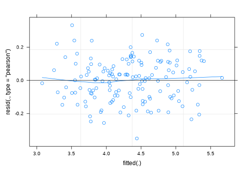<!-- --> --- # Assumption Plots: qqplots ```r library(lattice) qqmath(model, id=.05) ``` 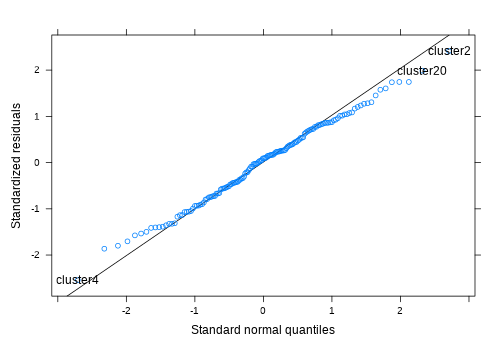<!-- --> --- # Assumption Plots: Scale-Location ```r plot(model, form = sqrt(abs(resid(.))) ~ fitted(.), type = c("p","smooth")) ``` 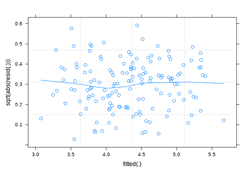<!-- --> --- count:false # Assumption Plots: Scale-Location ```r plot(model, form = sqrt(abs(resid(.))) ~ fitted(.) | cluster, type = c("p","smooth")) ``` <!-- --> --- # Assumption Plots: Ranefs .pull-left[ ```r qqmath(ranef(model)) ``` ``` ## $cluster ``` <!-- --> ] .pull-right[ ```r rans <- as.data.frame(ranef(model)$cluster) ggplot(rans, aes(sample = `(Intercept)`)) + stat_qq() + stat_qq_line() + labs(title="random intercept") ggplot(rans, aes(sample = x1)) + stat_qq() + stat_qq_line() labs(title="random slope") ``` <!-- --> ] --- # for a quick check if nothing else... ```r sjPlot::plot_model(model, type = "diag") ``` <!-- --> --- class: inverse, center, middle <h2><b style="opacity:0.4;">Part 1: Assumptions </b><b>Troubleshooting</b></h2> <h2 style="text-align: left;opacity:0.3;">Part 2: Case Diagnostics in MLM</h2> <h2 style="text-align: left;opacity:0.3;">Part 3: Random Effect Structures</h2> --- # Some Data .pull-left[ > 200 pupils from 20 schools completed a survey containing the Emotion Dysregulation Scale (EDS) and the Child Routines Questionnaire (CRQ). Eleven of the schools were taking part in an initiative to specifically teach emotion regulation as part of the curriculum. >Adjusting for levels of daily routines, do children from schools partaking in the intervention present with lower levels of emotional dysregulation? ] .pull-right[ <!-- --> ] --- # When things look wrong ```r mymodel <- lmer(emot_dysreg ~ crq + int + (1 | schoolid), data = crq) ``` <!-- --> --- # When things look wrong ### __Model mis-specification?__ .pull-left[ ```r mymodel <- lmer(emot_dysreg ~ crq + int + (1 | schoolid), data = crq) ``` <!-- --> ] .pull-right[ ```r mymodel <- lmer(emot_dysreg ~ crq + age + int + (1 | schoolid), data = crq) ``` <!-- --> ] --- # When things look wrong ### __Transformations?__ - Transforming your outcome variable may help to satisfy model assumptions -- - log(y) - 1/y - sqrt(y) - forecast::BoxCox(y) --- count:false # When things look wrong ### __Transformations?__ - Transforming your outcome variable may help to satisfy model assumptions .pull-left[ ```r lmer(y ~ x1 + g + (1 | cluster), df) ``` <!-- --> ] .pull-right[ ```r lmer(forecast::BoxCox(y,lambda="auto") ~ x1 + g + (1 | cluster), df) ``` <!-- --> ] --- count:false # When things look wrong ### __Transformations?__ - Transforming your outcome variable may help to satisfy model assumptions **but it comes at the expense of interpretability.** .pull-left[ ```r lmer(y ~ x1 + g + (1 | cluster), df) ``` ``` ## (Intercept) x1 g ## 36.137 1.615 10.020 ``` ] .pull-right[ ```r lmer(forecast::BoxCox(y,lambda="auto") ~ x1 + g + (1 | cluster), df) ``` ``` ## (Intercept) x1 g ## 1.733760 0.006857 0.048426 ``` ] --- count:false class: extra exclude: TRUE # When things look wrong ### __robustlmm__ .pull-left[ ```r mymodel <- lmer(emot_dysreg ~ crq * int + age + (1 | schoolid), data = crq) summary(mymodel)$coefficients ``` ``` ## Estimate Std. Error t value ## (Intercept) 1.0570 0.148701 7.108 ## crq -0.1338 0.018791 -7.119 ## intTreatment -0.3300 0.147007 -2.245 ## age 0.2720 0.007679 35.425 ## crq:intTreatment 0.0676 0.026673 2.534 ``` ] .pull-right[ ```r library(robustlmm) mymodelr <- rlmer(emot_dysreg ~ crq * int + age + (1 | schoolid), data = crq) summary(mymodelr)$coefficients ``` ``` ## Estimate Std. Error t value ## (Intercept) 1.01142 0.153154 6.604 ## crq -0.13198 0.018039 -7.317 ## intTreatment -0.33984 0.159706 -2.128 ## age 0.27408 0.007374 37.171 ## crq:intTreatment 0.07173 0.025609 2.801 ``` ] --- # When things look wrong ### __Bootstrap?__ basic idea: 1. do many many times:  a. take a sample (e.g. sample with replacement from your data, or simulated from your model parameters)  b. fit the model to the sample 2. then:  a. based on all the models fitted in step 1, obtain a distribution of parameter estimate of interest.  b. based on the bootstrap distribution from 2a, compute a confidence interval for estimate.  c. celebrate --- # Bootstrap: What do we (re)sample? resample based on the estimated distributions of parameters? - assumes explanatory variables are fixed, model specification and the distributions (e.g. `\(\zeta \sim N(0,\sigma_{\zeta})\)` and `\(\varepsilon \sim N(0,\sigma_{\varepsilon})\)`) are correct. -- resample residuals - `\(y* = \hat{y} + \hat{\varepsilon}_{\textrm{sampled with replacement}}\)` - assumes explanatory variables are fixed, and model specification is correct. -- resample cases - **minimal** assumptions - that we have correctly specified the hierarchical structure of data - **But** do we resample: - observations? - clusters? - both? --- # Bootstrap: Parametric ```r reducedmodel <- lmer(emot_dysreg ~ crq + age + (1 | schoolid), data = crq) mymodel <- lmer(emot_dysreg ~ crq + age + int + (1 | schoolid), data = crq) ``` - bootstrap LRT ```r library(pbkrtest) PBmodcomp(mymodel, reducedmodel) ``` - bootstrap CIs ```r confint(mymodel, method="boot") ``` -- - __lmeresampler__ package bootstrap() function ```r library(lmeresampler) mymodelBS <- bootstrap(mymodel, .f = fixef, type = "parametric", B = 2000) confint(mymodelBS, type = "norm") ``` .footnote[At time of writing, there is a minor bug with the version of **lmeresampler** that you can download from CRAN, so we recommend installing directly from the package maintainer: `devtools::install_github("aloy/lmeresampler")`] --- # Bootstrap: Cases ```r mymodel <- lmer(emot_dysreg ~ crq + age + int + (1 | schoolid), data = crq) ``` .pull-left[ ```r # devtools::install_github("aloy/lmeresampler") library(lmeresampler) # resample only children, not schools mymodelBScase <- bootstrap(mymodel, .f = fixef, type = "case", B = 2000, resample = c(FALSE, TRUE)) summary(mymodelBScase) ``` ``` ## Bootstrap type: case ## ## Number of resamples: 2000 ## ## term observed rep.mean se bias ## 1 (Intercept) 0.9563 0.9514 0.106136 -0.0049006 ## 2 crq -0.1004 -0.1007 0.013939 -0.0003475 ## 3 age 0.2727 0.2731 0.007825 0.0004362 ## 4 intTreatment -0.1520 -0.1525 0.024481 -0.0005422 ## ## There were 0 messages, 0 warnings, and 0 errors. ``` ] .pull-right[ ```r confint(mymodelBScase, type = "basic") ``` ``` ## # A tibble: 4 × 6 ## term estimate lower upper type level ## <chr> <dbl> <dbl> <dbl> <chr> <dbl> ## 1 (Intercept) 0.956 0.747 1.17 basic 0.95 ## 2 crq -0.100 -0.129 -0.0731 basic 0.95 ## 3 age 0.273 0.257 0.288 basic 0.95 ## 4 intTreatment -0.152 -0.199 -0.104 basic 0.95 ``` ] .footnote[<br>For a nice how-to guide on the **lmeresampler** package, see http://aloy.github.io/lmeresampler/articles/lmeresampler-vignette.html. For a discussion of different bootstrap methods for multilevel models, see Leeden R.., Meijer E., Busing F.M. (2008) Resampling Multilevel Models. In: Leeuw J.., Meijer E. (eds) Handbook of Multilevel Analysis. Springer, New York, NY. DOI: 10.1007/978-0-387-73186-5_11 ] --- count:false # Bootstrap: Cases ```r mymodel <- lmer(emot_dysreg ~ crq + age + int + (1 | schoolid), data = crq) ``` .pull-left[ ```r # devtools::install_github("aloy/lmeresampler") library(lmeresampler) # resample only children, not schools mymodelBScase <- bootstrap(mymodel, .f = fixef, type = "case", B = 2000, resample = c(FALSE, TRUE)) summary(mymodelBScase) ``` ``` ## Bootstrap type: case ## ## Number of resamples: 2000 ## ## term observed rep.mean se bias ## 1 (Intercept) 0.9563 0.9514 0.106136 -0.0049006 ## 2 crq -0.1004 -0.1007 0.013939 -0.0003475 ## 3 age 0.2727 0.2731 0.007825 0.0004362 ## 4 intTreatment -0.1520 -0.1525 0.024481 -0.0005422 ## ## There were 0 messages, 0 warnings, and 0 errors. ``` ] .pull-right[ ```r plot(mymodelBScase,"intTreatment") ``` <!-- --> ] .footnote[<br>For a nice how-to guide on the **lmeresampler** package, see http://aloy.github.io/lmeresampler/articles/lmeresampler-vignette.html. For a discussion of different bootstrap methods for multilevel models, see Leeden R.., Meijer E., Busing F.M. (2008) Resampling Multilevel Models. In: Leeuw J.., Meijer E. (eds) Handbook of Multilevel Analysis. Springer, New York, NY. DOI: 10.1007/978-0-387-73186-5_11 ] --- # Summary - Our assumptions for multi-level models are similar to that of a standard linear model in that we are concerned with the our residuals - in the multi-level case, we have residuals are multiple levels. - When assumptions appear violated, there are various courses of action to consider. - primarily, we should think about whether our model makes theoretical sense - Resampling methods (e.g. Bootstrapping) can be used to obtain confidence intervals and bias-corrected estimates of model parameters. - There are various forms of the bootstrap, with varying assumptions. --- class: inverse, center, middle, animated, rotateInDownLeft # End of Part 1 --- class: inverse, center, middle <h2 style="text-align: left;opacity:0.3;">Part 1: Assumptions</h2> <h2>Part 2: Case Diagnostics in MLM</h2> <h2 style="text-align: left;opacity:0.3;">Part 3: Random Effect Structures</h2> --- # Influence Just like standard `lm()`, observations can have unduly high influence on our model through a combination of high leverage and outlyingness. <img src="03_assumptdiag_files/figure-html/unnamed-chunk-45-1.png" style="display: block; margin: auto;" /> --- # multiple levels... - Both observations (level 1 units) __and__ clusters (level 2+ units) can be influential. -- - several packages, but current recommendation is **HLMdiag:** http://aloy.github.io/HLMdiag/index.html --- # Level 1 influential points .pull-left[ ```r mymodel <- lmer(emot_dysreg ~ crq + age + int + (1 | schoolid), data = crq) qqmath(mymodel, id=0.05) ``` <!-- --> ] -- .pull-right[ ```r library(HLMdiag) infl1 <- hlm_influence(mymodel, level = 1) names(infl1) ``` ``` ## [1] "id" "emot_dysreg" "crq" "age" ## [5] "int" "schoolid" "cooksd" "mdffits" ## [9] "covtrace" "covratio" "leverage.overall" ``` ```r infl1 ``` ``` ## # A tibble: 174 × 11 ## id emot_dysreg crq age int schoolid cooksd mdffits covtrace ## <int> <dbl> <dbl> <dbl> <fct> <fct> <dbl> <dbl> <dbl> ## 1 1 4.12 1.92 14 Treatment school1 0.0000660 6.59e-5 0.000869 ## 2 2 3.22 1.65 11 Treatment school1 0.00749 7.34e-3 0.0194 ## 3 3 4.86 3.56 16 Treatment school1 0.0185 1.80e-2 0.0252 ## 4 4 4.79 1.45 16 Treatment school1 0.0000195 1.92e-5 0.0169 ## 5 5 3.58 0.81 12 Treatment school1 0.00692 6.79e-3 0.0185 ## 6 6 4.41 2.71 15 Treatment school1 0.00000410 4.07e-6 0.00601 ## 7 7 4.23 3.01 14 Treatment school1 0.00104 1.04e-3 0.00620 ## 8 8 3.66 1.61 12 Treatment school1 0.000102 1.01e-4 0.00897 ## 9 9 4.22 2.17 14 Treatment school1 0.00000750 7.50e-6 0.000568 ## 10 10 4.42 2.28 14 Treatment school2 0.000254 2.53e-4 0.00466 ## # … with 164 more rows, and 2 more variables: covratio <dbl>, ## # leverage.overall <dbl> ``` ] --- count:false # Level 1 influential points .pull-left[ ```r mymodel <- lmer(emot_dysreg ~ crq + age + int + (1 | schoolid), data = crq) qqmath(mymodel, id=0.05) ``` <!-- --> ] .pull-right[ ```r library(HLMdiag) infl1 <- hlm_influence(mymodel, level = 1) dotplot_diag(infl1$cooksd, cutoff = "internal") ``` <!-- --> ] --- # Level 2 influential clusters ```r infl2 <- hlm_influence(mymodel, level = "schoolid") dotplot_diag(infl2$cooksd, cutoff = "internal", index=infl2$schoolid) ``` <!-- --> --- # What to do? - In this context (children from schools), I would be inclined not to worry too much about the individual children who have high values on cook's distance, __if__ we plan on case-based bootstrap for our inferential tests (and plan on resampling the level 1 units - the children). -- - It's worth looking into school 6 a bit further. - `mdffits` is a measure of multivariate "difference in fixed effects" ```r infl2 %>% arrange(desc(mdffits)) ``` ``` ## # A tibble: 20 × 6 ## schoolid cooksd mdffits covtrace covratio leverage.overall ## <fct> <dbl> <dbl> <dbl> <dbl> <dbl> ## 1 school6 0.369 0.330 0.253 1.27 0.107 ## 2 school8 0.144 0.128 0.245 1.26 0.131 ## 3 school17 0.134 0.121 0.267 1.29 0.108 ## 4 school1 0.112 0.104 0.193 1.20 0.117 ## 5 school4 0.116 0.103 0.267 1.29 0.111 ## 6 school5 0.108 0.0992 0.239 1.26 0.129 ## 7 school11 0.107 0.0990 0.229 1.24 0.110 ## 8 school7 0.0767 0.0701 0.283 1.31 0.148 ## 9 school18 0.0730 0.0675 0.118 1.12 0.126 ## 10 school16 0.0680 0.0620 0.195 1.21 0.122 ## 11 school15 0.0522 0.0503 0.185 1.19 0.122 ## 12 school20 0.0451 0.0426 0.242 1.26 0.105 ## 13 school2 0.0427 0.0411 0.148 1.15 0.171 ## 14 school9 0.0420 0.0405 0.186 1.20 0.122 ## 15 school12 0.0281 0.0259 0.256 1.28 0.126 ## 16 school14 0.0265 0.0255 0.208 1.22 0.106 ## 17 school3 0.0129 0.0116 0.218 1.23 0.118 ## 18 school19 0.0100 0.00949 0.246 1.27 0.108 ## 19 school13 0.00844 0.00784 0.197 1.21 0.120 ## 20 school10 0.00578 0.00559 0.199 1.21 0.237 ``` --- count:false # What to do? - In this context (children from schools), I would be inclined not to worry too much about the individual children who have high values on cook's distance, __if__ we plan on bootstrapping our inferential tests (and plan on resampling the level 1 units - the children). - It's worth looking into school 6 a bit further. - examine fixed effects upon deletion of schools 6 ```r delete6 <- case_delete(mymodel, level = "schoolid", type = "fixef", delete = "school6") cbind(delete6$fixef.original, delete6$fixef.delete) ``` ``` ## [,1] [,2] ## (Intercept) 0.9563 1.06034 ## crq -0.1004 -0.08985 ## age 0.2727 0.26519 ## intTreatment -0.1520 -0.18202 ``` --- # Sensitivity Analysis? Would our conclusions change if we excluded these schools? ```r mymodelrm6 <- lmer(emot_dysreg ~ crq + age + int + (1 | schoolid), data = crq %>% filter(!schoolid %in% c("school6"))) mymodelrm6BS <- bootstrap(mymodelrm6, .f = fixef, type = "case", B = 2000, resample = c(FALSE, TRUE)) confint(mymodelrm6BS, type = "basic") ``` ``` ## # A tibble: 4 × 6 ## term estimate lower upper type level ## <chr> <dbl> <dbl> <dbl> <chr> <dbl> ## 1 (Intercept) 1.06 0.857 1.26 basic 0.95 ## 2 crq -0.0899 -0.117 -0.0627 basic 0.95 ## 3 age 0.265 0.251 0.280 basic 0.95 ## 4 intTreatment -0.182 -0.229 -0.136 basic 0.95 ``` --- # Summary - Influence can be exerted by individual observations and higher lever groups of observations - e.g. by children and by schools, or by individual trials and by participants. - We can get measures of influence at different levels, and consider how estimates and conclusions might change when certain observations (or groups) are excluded - Bootstrapping is relevant as whether we are resampling at the level of an influential group/observation is going to affect the extent to which our estimates are biased by that observation/group --- class: inverse, center, middle, animated, rotateInDownLeft # End of Part 3 --- class: inverse, center, middle <h2 style="text-align: left;opacity:0.3;">Part 1: Assumptions</h2> <h2 style="text-align: left;opacity:0.3;">Part 2: Case Diagnostics in MLM</h2> <h2>Part 3: Random Effect Structures</h2> --- # What have we seen so far? - children within schools - birds within gardens - measurements within participants - nurses within hospitals - and probably some others... --- # Nested - the level `\(j\)` observations in a level `\(i\)` group belong __only__ to that level `\(i\)` group. <img src="https://media.gettyimages.com/photos/albatross-chick-between-parents-feet-falkland-islands-picture-id642348358?s=2048x2048" width="450px" style="display: block; margin: auto;" /> --- count:false # Nested - the level `\(j\)` observations in a level `\(i\)` group belong __only__ to that level `\(i\)` group. - __`(1 | school/class)`__ or __`(1 | school) + (1 | class:school)`__ <img src="jk_img_sandbox/structure_id.png" width="1460" style="display: block; margin: auto;" /> --- count:false # Nested - the level `\(j\)` observations in a level `\(i\)` group belong __only__ to that level `\(i\)` group. - If labels are unique, __`(1 | school) + (1 | class)`__ is the same as __`(1 | school/class)`__ <img src="jk_img_sandbox/structure_nested.png" width="1460" style="display: block; margin: auto;" /> --- # Crossed - "crossed" = not nested! -- - __`(1 | subject) + (1 | task)`__ <img src="jk_img_sandbox/structure_crossed.png" width="668" height="450px" style="display: block; margin: auto;" /> --- # Fixed or random .pull-left[ | Criterion: | Repetition: <br> _If the experiment were repeated:_ | Desired inference: <br> _The conclusions refer to:_ | |----------------|--------------------------------------------------|----------------------------------------------------| | Fixed effects | <center>Same levels would be used</center> | <center>The levels used </center> | | Random effects | <center>Different levels would be used</center> | <center>A population from which the levels used<br> are just a (random) sample</center> | ] .pull-right[ - If only small number of clusters, estimating variance components may be unstable. - Partialling out cluster-differences as fixed effects *may* be preferable. ] --- # Maximal Structures - "maximal" = the most complex random effect structure that you can fit to the data -- - requires sufficient variance at all levels (for both intercepts and slopes where relevant). Which is often not the case. -- ```r maxmodel <- lmer(emot_dysreg ~ crq + age + int + (1 + crq + age | schoolid), data = crq) ``` ``` ## Warning in checkConv(attr(opt, "derivs"), opt$par, ctrl = control$checkConv, : ## Model failed to converge with max|grad| = 0.00275817 (tol = 0.002, component 1) ``` -- another example: 16 items each occur in 4 different combinations: condition A vs B `\(\times\)` type 1 vs 2. 40 participants see all items in all conditions (64 trials each participant). ```r mmod <- lmer(outcome ~ condition * type + (1 + condition * type | ppt) + (1 + condition * type | item), data = kelly) ``` ``` ## boundary (singular) fit: see ?isSingular ``` --- # Model Convergence - Don't report results from a model that doesn't converge. You will probably not be able to trust the estimates. -- - Try a different optimiser, adjust the max iterations, or the stopping tolerances <img src="jk_img_sandbox/tolerance.png" width="557" /> --- count:false # Model Convergence - Don't report results from a model that doesn't converge. You will probably not be able to trust the estimates. - Try a different optimiser, adjust the max iterations, or the stopping tolerances <br><br> - Remove random effects with least variance until model converges (see Barr et al., 2013) - Use a criterion for model selection (e.g. AIC, BIC) to choose a random effect structure that is supported by the data (see Matsuchek et al., 2017) -- - __No right answer__ --- # correlations between random effects ``` ## Groups Name Std.Dev. Corr ## ppt (Intercept) 91.7 ## conditionB 59.1 -0.21 ## type2 27.6 0.25 -0.42 ## conditionB:type2 22.4 -0.32 -0.86 0.26 ## item (Intercept) 37.0 ## conditionB 35.8 -0.18 ## type2 20.2 0.14 -0.40 ## conditionB:type2 65.6 0.25 0.27 -0.92 ## Residual 203.2 ``` --- count:false # correlations between random effects .pull-left[ __perfect correlations__ ```r m1 <- lmer(y ~ 1 + x1 + (1 + x1 | clusterid), data = df) VarCorr(m1) ``` ``` ## Groups Name Std.Dev. Corr ## clusterid (Intercept) 0.759 ## x1 0.117 1.00 ## Residual 0.428 ``` ``` ## $clusterid ``` <!-- --> ] -- .pull-right[ <!-- --> ] --- count:false # correlations between random effects .pull-left[ __perfect correlations__ ```r m1 <- lmer(y ~ 1 + x1 + (1 + x1 | clusterid), data = df) VarCorr(m1) ``` ``` ## Groups Name Std.Dev. Corr ## clusterid (Intercept) 0.759 ## x1 0.117 1.00 ## Residual 0.428 ``` ``` ## $clusterid ``` <!-- --> ] .pull-right[ __zero correlations__ ```r zcpmodel <- lmer(y ~ 1 + x1 + (1 + x1 || clusterid), data = df) VarCorr(zcpmodel) ``` ``` ## Groups Name Std.Dev. ## clusterid (Intercept) 0.751 ## clusterid.1 x1 0.104 ## Residual 0.432 ``` ``` ## $clusterid ``` <!-- --> ] --- # correlations between random effects When should we remove them? -- __When it makes theoretical sense to do so.__ --- # Summary - random effect structures can get complicated quite quickly - we can have multiple levels of nesting - we can have crossed random effects - the maximal random effect structure is the most complex structure we can fit to the data. - it often leads to problems with model convergence - building MLMs is a balancing act between accounting for different sources of variance and attempting to fit a model that is too complex for our data. --- class: inverse, center, middle, animated, rotateInDownLeft # End