Multilevel Models

class: center, middle, inverse, title-slide

# <b>Multilevel Models</b>
## Data Analysis for Psychology in R 3
### Josiah King, Umberto Noè, Tom Booth
### Department of Psychology<br/>The University of Edinburgh
### AY 2021-2022

---

class: inverse, center, middle

<h2>Part 1: LM to MLM</h2>
<h2 style="text-align: left;opacity:0.3;">Part 2: Inference in MLM</h2>

---
# Terminology

<div class="figure" style="text-align: center">
<img src="jk_img_sandbox/mlmname.png" alt="(size weighted by hits on google scholar)" width="827" />
<p class="caption">(size weighted by hits on google scholar)</p>
</div>

---
# Notation 







**Simple regression**  
.pull-left[
`$\begin{align} & \text{for observation }i \\ \quad \\ \quad \\ & \color{red}{y_i} = \color{blue}{\beta_0 \cdot{} 1 \; + \; \beta_1 \cdot{} x_{i} } + \varepsilon_i \\ \end{align}$`
]

---
# Notation

**Multi-level**  
.pull-left[
`$\begin{align} & \text{for observation }j\text{ in group }i \\ \quad \\ & \text{Level 1:} \\ & \color{red}{y_{ij}} = \color{blue}{\beta_{0i} \cdot 1 + \beta_{1i} \cdot x_{ij}} + \varepsilon_{ij} \\ & \text{Level 2:} \\ & \color{blue}{\beta_{0i}} = \gamma_{00} + \color{orange}{\zeta_{0i}} \\ & \color{blue}{\beta_{1i}} = \gamma_{10} + \color{orange}{\zeta_{1i}} \\ \quad \\ \end{align}$`
]

.pull-right[
`$\begin{align} & \text{Where:} \\ & \gamma_{00}\text{ is the population intercept}\\ & \text{and  }\color{orange}{\zeta_{0i}}\text{ is the deviation of group }i\text{ from }\gamma_{00} \\ \qquad \\ & \gamma_{10}\text{ is the population slope,}\\ & \text{and }\color{orange}{\zeta_{1i}}\text{ is the deviation of group }i\text{ from }\gamma_{10} \\ \end{align}$`
]

We are now assuming `$\color{orange}{\zeta_0}$`, `$\color{orange}{\zeta_1}$`, and `$\varepsilon$` to be normally distributed with a mean of 0, and we denote their variances as `$\sigma_{\color{orange}{\zeta_0}}^2$`, `$\sigma_{\color{orange}{\zeta_1}}^2$`, `$\sigma_\varepsilon^2$` respectively.

The `$\color{orange}{\zeta}$` components also get termed the "random effects" part of the model, Hence names like "random effects model", etc.

---
# Notation

**Mixed-effects == Multi Level**

Sometimes, you will see the levels collapsed into one equation, as it might make for more intuitive reading:

`$\color{red}{y_{ij}} = \underbrace{(\gamma_{00} + \color{orange}{\zeta_{0i}})}_{\color{blue}{\beta_{0i}}} \cdot 1 + \underbrace{(\gamma_{10} + \color{orange}{\zeta_{1i}})}_{\color{blue}{\beta_{1i}}} \cdot x_{ij}  +  \varepsilon_{ij} \\$`

.footnote[
**other notation to be aware of**

- Many people use the symbol `$u$` in place of `$\zeta$`

- Sometimes people use `$\beta_{00}$` instead of `$\gamma_{00}$`

- In various resources, you are likely to see `$\alpha$` used to denote the intercept instead of `$\beta_0$`

]

---
count:false
class: extra
exclude: FALSE
# Notation

__Matrix form__

And then we also have the condensed matrix form of the model, in which the Z matrix represents the grouping structure of the data, and `$\zeta$` contains the estimated random deviations.

`$\begin{align} \color{red}{\begin{bmatrix} y_{11} \\ y_{12} \\ y_{21} \\ y_{22} \\ y_{31} \\ y_{32} \\ \end{bmatrix}} & = \color{blue}{\begin{bmatrix} 1 & x_{11} \\ 1 & x_{12} \\ 1 & x_{21} \\ 1 & x_{22} \\1 & x_{31} \\ 1 & x_{32} \\ \end{bmatrix} \begin{bmatrix} \gamma_{00} \\ \beta_1 \\  \end{bmatrix}} & + & \color{orange}{ \begin{bmatrix} 1 & 0 & 0 \\ 1 & 0 & 0 \\ 0 & 1 & 0 \\ 0 & 1 & 0 \\ 0 & 0 & 1 \\ 0 & 0 & 1 \\ \end{bmatrix} \begin{bmatrix}\zeta_{01} \\ \zeta_{02} \\ \zeta_{03} \end{bmatrix}} & + & \begin{bmatrix} \varepsilon_{11} \\ \varepsilon_{12} \\ \varepsilon_{21} \\ \varepsilon_{22} \\ \varepsilon_{31} \\ \varepsilon_{32} \end{bmatrix} \\ \qquad \\ \\ \color{red}{\boldsymbol y}\;\;\;\;\; & = \qquad \mathbf{\color{blue}{X \qquad \;\;\boldsymbol \beta}} & + & \qquad \; \mathbf{\color{orange}{Z \qquad \;\;\;\;\; \boldsymbol \zeta}} & + & \;\;\;\varepsilon \\ \end{align}$`

---
# "Fixed" vs "Random"

.pull-left[
`$\begin{align}& \text{Level 1:} \\ & \color{red}{y_{ij}} = \color{blue}{\beta_{0i} \cdot 1 + \beta_{1i} \cdot x_{ij}} + \varepsilon_{ij} \\ & \text{Level 2:} \\ & \color{blue}{\beta_{0i}} = \underbrace{\gamma_{00}}_{\textrm{fixed}} + \color{orange}{\underbrace{\zeta_{0i}}_{\textrm{random}}} \\ & \color{blue}{\beta_{1i}} = \underbrace{\gamma_{10}}_{\textrm{fixed}} + \color{orange}{\underbrace{\zeta_{1i}}_{\textrm{random}}} \\ \quad \\ \end{align}$`
]
.pull-right[
`$\color{red}{y_{ij}} = (\underbrace{\gamma_{00}}_{\textrm{fixed}} + \color{orange}{\underbrace{\zeta_{0i}}_{\textrm{random}}}) \cdot 1 + (\underbrace{\gamma_{10}}_{\textrm{fixed}} + \color{orange}{\underbrace{\zeta_{1i}}_{\textrm{random}}}) \cdot x_{ij}  +  \varepsilon_{ij} \\$`
]

`$\color{orange}{\zeta_i}$` is "random" because considered a random sample from larger population such that `$\color{orange}{\zeta_i} \sim N(0, \sigma^2_{\color{orange}{\zeta_i}})$`.

---
# Fixed vs Random

What is the difference?

When specifying a random effects model, think about the data you have and how they fit in the following table:

| Criterion: | Repetition: <br> _If the experiment were repeated:_ | Desired inference: <br> _The conclusions refer to:_ |
|----------------|--------------------------------------------------|----------------------------------------------------|
| Fixed effects  | <center>Same levels would be used</center>     |    <center>The levels used </center>                                   |
| Random effects | <center>Different levels would be used</center>   | <center>A population from which the levels used<br> are just a (random) sample</center> |

- Sometimes, there isn't much variability in a specific random effect and to allow your model to fit it is common to just model that variable as a fixed effect.

- Other times, you don't have sufficient data or levels to estimate the random effect variance, and you are forced to model it as a fixed effect.

---
# Advantages of MLM

Multi-level models can be used to answer multi-level questions!  
<br><br>
Do phenomena at Level X predict __outcomes__ at Level Y?

.pull-left[
Does population density in school district predict variation in scores in childrens' first year of school?  
]
.pull-right[
`$\textrm{score}_{ij} = \beta_{0i} + \beta_1\textrm{school_year}_j + \varepsilon_{ij}$`  
<br>
`$\beta_{0i} = \gamma_{00} + \gamma_{01}\textrm{district_pop_dens}_i + \zeta_{0i}$`  
]

---
# Advantages of MLM

Multi-level models can be used to answer multi-level questions!  
<br><br>
Do phenomena at Level X influence __effects__ at Level Y?

.pull-left[
Does amount of school funding influence childrens' improvement in scores over time?  
]
.pull-right[
`$\textrm{score}_{ij} = \beta_{0} + \beta_{1i}\textrm{school_year}_j + \varepsilon_{ij}$`  
<br>
`$\beta_{1i} = \gamma_{10} + \gamma_{11}\textrm{school_funding}_i + \zeta_{1i}$`
]
  
---
# Advantages of MLM

Multi-level models can be used to answer multi-level questions!  
<br><br>
Do random variances covary?

.pull-left[
Do children who score higher at the start of school show greater improvements than those who start lower?  
]
.pull-right[
`$\textrm{score}_{ij} = \beta_{0i} + \beta_{1i}\textrm{school_year}_j + \varepsilon_{ij}$`  
<br>
`$\beta_{0i} = \gamma_{00} + \zeta_{0i}$`  
`$\beta_{1i} = \gamma_{10} + \zeta_{1i}$`  
<br>
$$
`\begin{bmatrix}
\sigma^2_{\zeta_{0}} & \\ \sigma_{\zeta_{0},\zeta_{1}} & \sigma^2_{\zeta_{1}} \\
\end{bmatrix}`
$$
]

---
# lme4

- **lme4** package (many others are available, but **lme4** is most popular).

- `lmer()` function.

- syntax is similar to `lm()`, in that we specify:

__*[outcome variable]*__ ~ __*[explanatory variables]*__, data = __*[name of dataframe]*__
    
- in `lmer()`, we add to this the random effect structure in parentheses:

__*[outcome variable]*__ ~ __*[explanatory variables]*__ + (__*[vary this]*__ | __*[by this grouping variable]*__), data = __*[name of dataframe]*__, REML = __*[TRUE/FALSE]*__

---
count:false
class: center, middle, animated, rotateInDownLeft

<b style="opacity:0.4;">take a break... </b>

---
class: inverse, center, middle

<h2><b style="opacity:0.4;">Part 1: LM to MLM </b><b>Estimation</b></h2>
<h2 style="text-align: left;opacity:0.3;">Part 2: Inference in MLM</h2>

---
# Model Estimation

- For standard linear models, we can calculate the parameters using a *closed form solution*.

- Multilevel models are too complicated, we *estimate* all the parameters using an iterative procedure like Maximum Likelihood Estimation (MLE).

---
# Model Estimation: MLE

Aim: find the values for the unknown parameters that maximize the probability of obtaining the observed data.
How: This is done via finding values for the parameters that maximize the (log) likelihood function.

---
count:false
class: extra
exclude: FALSE
# Model Estimation: (log)Likelihood

- Data = multiple observations: `$1, ..., n$`

- From our axioms of probability, we can combine these *i.i.d* by multiplication to get our likelihood of our parameters given our entire sample

- Instead of taking the **product** of the individual likelihoods, we can take the **summation** of the log-likelihoods
    - This is considerably easier to do, and can be achieved because multiplication is addition on a log scale.

---
# Model Estimation: MLE

In multilevel models, our parameter space is more complex (e.g. both fixed effects and variance components).

---
# Model Estimation: ML vs REML

- Standard ML results in biased estimates of variance components.

- Restricted Maximum Likelihood (REML) is the default in `lmer()`.

- REML separates the estimation of fixed and random parts of the model, leading to less biased estimates of the variance components.

- **Use ML to compare models that differ in their fixed effects.**

---
count:false
class: center, middle, animated, rotateInDownLeft

<b style="opacity:0.4;">take a break... </b>

---
class: inverse, center, middle

<h2><b style="opacity:0.4;">Part 1: LM to MLM </b><b>A Visual Explanation</b></h2>
<h2 style="text-align: left;opacity:0.3;">Part 2: Inference in MLM</h2>

---
# Data

.pull-left[

> 200 pupils from 20 schools completed a survey containing the Emotion Dysregulation Scale (EDS) and the Child Routines Questionnaire (CRQ).

]
.pull-right[

```r
crq <- read_csv("https://uoepsy.github.io/data/crqdata.csv")
head(crq)
```

```
## # A tibble: 6 × 6
##   emot_dysreg   crq int       schoolid sleep   age
##         <dbl> <dbl> <chr>     <chr>    <chr> <dbl>
## 1        4.12  1.92 Treatment school1  <8hr     14
## 2        3.22  1.65 Treatment school1  <8hr     11
## 3        4.86  3.56 Treatment school1  <8hr     16
## 4        4.79  1.45 Treatment school1  8hr+     16
## 5        3.58  0.81 Treatment school1  <8hr     12
## 6        4.41  2.71 Treatment school1  <8hr     15
```
]

---
count: false
# Data

.pull-left[

> 200 pupils from 20 schools completed a survey containing the Emotion Dysregulation Scale (EDS) and the Child Routines Questionnaire (CRQ).

```r
schoolplots <- 
  ggplot(crq, aes(x = crq, y = emot_dysreg, 
                  col = schoolid)) +
  geom_point()+
  facet_wrap(~schoolid) + 
  guides(col = "none") +
  labs(x = "Child Routines Questionnaire (CRQ)", 
       y = "Emotion Dysregulation Scale (EDS)") +
  themedapr3()
```
]
.pull-right[

```r
schoolplots
```

![](02_intromlm_files/figure-html/unnamed-chunk-7-1.png)

]

---
# ICC

.pull-left[

```r
library(ggridges)
ggplot(crq, aes(x = emot_dysreg, y = schoolid, 
                fill = schoolid)) +
  geom_density_ridges(jittered_points = TRUE, 
                      position = "raincloud", alpha = .4,
                      quantile_lines=TRUE,
                      quantile_fun=function(x,...) mean(x)) +
  guides(fill=FALSE) + 
  themedapr3()
```

![](02_intromlm_files/figure-html/unnamed-chunk-8-1.png)
]
.pull-right[

```r
library(ICC)
ICCbare(schoolid, emot_dysreg, data = crq)
```

```
## [1] 0.2443
```

__Reminder:__ the Intraclass Correlation Coefficient is ratio of variance between clusters to the total variance (variance within + variance between).

]

---
# R: fitting lm

.pull-left[

```r
lm_mod <- lm(emot_dysreg ~ 1 + crq, data = crq)
summary(lm_mod)
```

```
## 
## Call:
## lm(formula = emot_dysreg ~ 1 + crq, data = crq)
## 
## Residuals:
##     Min      1Q  Median      3Q     Max 
## -1.1643 -0.4667  0.0158  0.4333  1.3338 
## 
## Coefficients:
##             Estimate Std. Error t value Pr(>|t|)    
*## (Intercept)   4.4470     0.1259   35.31   <2e-16 ***
*## crq          -0.0525     0.0448   -1.17     0.24    
## ---
## Signif. codes:  0 '***' 0.001 '**' 0.01 '*' 0.05 '.' 0.1 ' ' 1
## 
## Residual standard error: 0.581 on 172 degrees of freedom
## Multiple R-squared:  0.00794,	Adjusted R-squared:  0.00217 
## F-statistic: 1.38 on 1 and 172 DF,  p-value: 0.242
```

]

.pull-right[

```r
schoolplots + 
  geom_line(aes(y=fitted(lm_mod)), col = "blue", lwd=1)
```

![](02_intromlm_files/figure-html/unnamed-chunk-11-1.png)

]

---
# R: Adding a random intercept

.pull-left[
vary the intercept by schools.

```r
library(lme4)
ri_mod <- lmer(emot_dysreg ~ 1 + crq + 
                 (1 | schoolid), data = crq)
summary(ri_mod)
```

```
## Linear mixed model fit by REML ['lmerMod']
## Formula: emot_dysreg ~ 1 + crq + (1 | schoolid)
##    Data: crq
## 
## REML criterion at convergence: 290.6
## 
## Scaled residuals: 
##     Min      1Q  Median      3Q     Max 
## -1.9203 -0.8709  0.0341  0.6536  2.3091 
## 
## Random effects:
##  Groups   Name        Variance Std.Dev.
*##  schoolid (Intercept) 0.0847   0.291   
##  Residual             0.2578   0.508   
## Number of obs: 174, groups:  schoolid, 20
## 
## Fixed effects:
##             Estimate Std. Error t value
*## (Intercept)   4.4299     0.1300   34.07
## crq          -0.0510     0.0402   -1.27
## 
## Correlation of Fixed Effects:
##     (Intr)
## crq -0.812
```

]

.pull-right[

```r
schoolplots + 
  geom_line(aes(y=fitted(lm_mod)), col = "blue", lwd=1) + 
  geom_line(aes(y=fitted(ri_mod)), col = "red", lwd=1)
```

![](02_intromlm_files/figure-html/unnamed-chunk-13-1.png)
]

---
# R: Adding a random slope

.pull-left[
vary the intercept and the effect (slope) of crq by schools

```r
rs_mod <- lmer(emot_dysreg ~ crq + 
                 (1 + crq | schoolid), data = crq)
summary(rs_mod)
```

```
## Linear mixed model fit by REML ['lmerMod']
## Formula: emot_dysreg ~ crq + (1 + crq | schoolid)
##    Data: crq
## 
## REML criterion at convergence: 288.6
## 
## Scaled residuals: 
##    Min     1Q Median     3Q    Max 
## -1.879 -0.836  0.041  0.644  2.051 
## 
## Random effects:
##  Groups   Name        Variance Std.Dev. Corr 
*##  schoolid (Intercept) 0.242    0.492         
*##           crq         0.019    0.138    -0.80
##  Residual             0.239    0.489         
## Number of obs: 174, groups:  schoolid, 20
## 
## Fixed effects:
##             Estimate Std. Error t value
*## (Intercept)   4.4377     0.1569   28.28
*## crq          -0.0517     0.0506   -1.02
## 
## Correlation of Fixed Effects:
##     (Intr)
## crq -0.873
```

]

.pull-right[

```r
schoolplots + 
  geom_line(aes(y=fitted(lm_mod)), col = "blue", lwd=1) + 
  geom_line(aes(y=fitted(ri_mod)), col = "red", lwd=1) + 
  geom_line(aes(y=fitted(rs_mod)), col = "orange", lwd=1)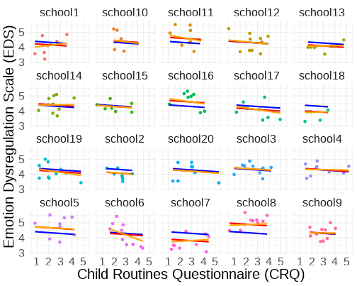
```

![](02_intromlm_files/figure-html/unnamed-chunk-15-1.png)
]

---
# Partial Pooling vs No Pooling

.pull-left[
Why not fit a fixed effect adjustment to the slope of x for each group?  
`lm(y ~ x * group)`?

```r
fe_mod <- lm(emot_dysreg ~ crq * schoolid, data = crq)
```
]

.pull-right[

```r
schoolplots + 
  geom_line(aes(y=fitted(fe_mod)), col = "black", lwd=1)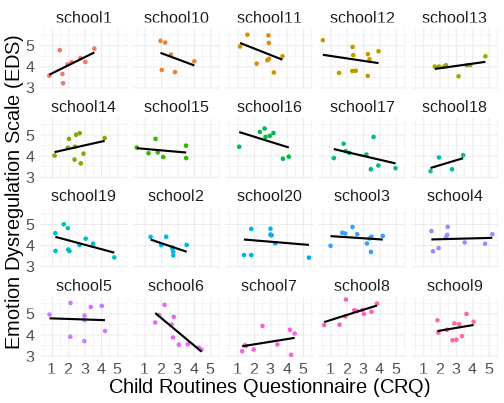
```

![](02_intromlm_files/figure-html/unnamed-chunk-17-1.png)
]

---
# Partial Pooling vs No Pooling

.pull-left[
- We talked last week about how this results in a lot of output. With 20 schools, we get: intercept at reference school, adjustment for every other school, the effect of x at reference school, adjustment to effect of x for every other school. 
    
    ```r
    length(coef(fe_mod))
    ```
    
    ```
    ## [1] 40
    ```
- information is not combined in anyway (data from school `$i$` contributes to differences from reference school to school `$i$`, but nothing else. No overall estimates)

]

.pull-right[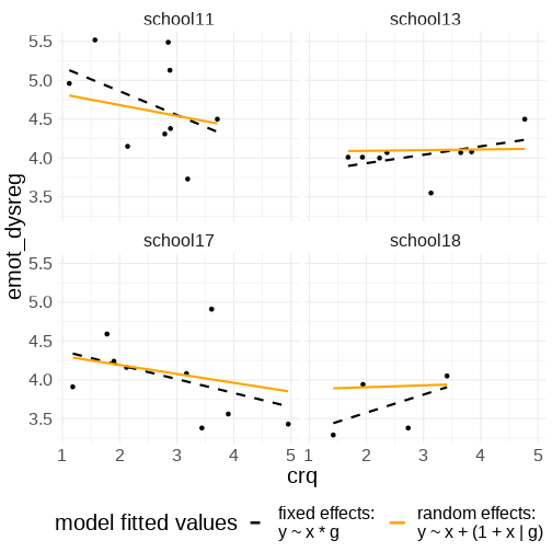
![](02_intromlm_files/figure-html/unnamed-chunk-19-1.png)
]

---
count:false
class: center, middle, animated, rotateInDownLeft

<b style="opacity:0.4;">take a break... </b>

---
class: inverse, center, middle

<h2><b style="opacity:0.4;">Part 1: LM to MLM </b><b>lme4 Output</b></h2>
<h2 style="text-align: left;opacity:0.3;">Part 2: Inference in MLM</h2>

---
# Understanding MLM output

.pull-left[

```
## Linear mixed model fit by REML ['lmerMod']
## Formula: y ~ x + (1 + x | group)
##    Data: my_data
## 
## REML criterion at convergence: 334.6
## 
## Scaled residuals: 
##     Min      1Q  Median      3Q     Max 
## -2.1279 -0.7009  0.0414  0.6645  2.1010 
## 
## Random effects:
##  Groups   Name        Variance Std.Dev. Corr 
##  group    (Intercept) 1.326    1.152         
##           x           0.152    0.390    -0.88
##  Residual             0.262    0.512         
## Number of obs: 170, groups:  group, 20
## 
## Fixed effects:
##             Estimate Std. Error t value
*## (Intercept)   1.7890     0.2858    6.26
*## x            -0.6250     0.0996   -6.27
```
]
.pull-right[
<img src="jk_img_sandbox/lmer2.png" width="1391" />
]

---
count: false
# Understanding MLM output

.pull-left[

```
## Linear mixed model fit by REML ['lmerMod']
## Formula: y ~ x + (1 + x | group)
##    Data: my_data
## 
## REML criterion at convergence: 334.6
## 
## Scaled residuals: 
##     Min      1Q  Median      3Q     Max 
## -2.1279 -0.7009  0.0414  0.6645  2.1010 
## 
## Random effects:
##  Groups   Name        Variance Std.Dev. Corr 
*##  group    (Intercept) 1.326    1.152         
*##           x           0.152    0.390    -0.88
##  Residual             0.262    0.512         
## Number of obs: 170, groups:  group, 20
## 
## Fixed effects:
##             Estimate Std. Error t value
## (Intercept)   1.7890     0.2858    6.26
## x            -0.6250     0.0996   -6.27
```
]
.pull-right[
<img src="jk_img_sandbox/lmer2a.png" width="1391" />
]

---
count: false
# Understanding MLM output

.pull-left[

```
## Linear mixed model fit by REML ['lmerMod']
## Formula: y ~ x + (1 + x | group)
##    Data: my_data
## 
## REML criterion at convergence: 334.6
## 
## Scaled residuals: 
##     Min      1Q  Median      3Q     Max 
## -2.1279 -0.7009  0.0414  0.6645  2.1010 
## 
## Random effects:
##  Groups   Name        Variance Std.Dev. Corr 
*##  group    (Intercept) 1.326    1.152         
*##           x           0.152    0.390    -0.88
##  Residual             0.262    0.512         
## Number of obs: 170, groups:  group, 20
## 
## Fixed effects:
##             Estimate Std. Error t value
*## (Intercept)   1.7890     0.2858    6.26
*## x            -0.6250     0.0996   -6.27
```
]
.pull-right[
<img src="jk_img_sandbox/lmer3.png" width="1391" />
]

---
count: false
# Understanding MLM output

.pull-left[

```
## Linear mixed model fit by REML ['lmerMod']
## Formula: y ~ x + (1 + x | group)
##    Data: my_data
## 
## REML criterion at convergence: 334.6
## 
## Scaled residuals: 
##     Min      1Q  Median      3Q     Max 
## -2.1279 -0.7009  0.0414  0.6645  2.1010 
## 
## Random effects:
##  Groups   Name        Variance Std.Dev. Corr 
##  group    (Intercept) 1.326    1.152         
##           x           0.152    0.390    -0.88
*##  Residual             0.262    0.512         
## Number of obs: 170, groups:  group, 20
## 
## Fixed effects:
##             Estimate Std. Error t value
## (Intercept)   1.7890     0.2858    6.26
## x            -0.6250     0.0996   -6.27
```
]
.pull-right[
<img src="jk_img_sandbox/lmer4.png" width="1391" />
]

---
# Extracting MLM output

.pull-left[

```
## Linear mixed model fit by REML ['lmerMod']
## Formula: y ~ x + (1 + x | group)
##    Data: my_data
## 
## REML criterion at convergence: 334.6
## 
## Scaled residuals: 
##     Min      1Q  Median      3Q     Max 
## -2.1279 -0.7009  0.0414  0.6645  2.1010 
## 
## Random effects:
##  Groups   Name        Variance Std.Dev. Corr 
##  group    (Intercept) 1.326    1.152         
##           x           0.152    0.390    -0.88
##  Residual             0.262    0.512         
## Number of obs: 170, groups:  group, 20
## 
## Fixed effects:
##             Estimate Std. Error t value
## (Intercept)   1.7890     0.2858    6.26
## x            -0.6250     0.0996   -6.27
```
]
.pull-right[

```r
fixef(model)
```

```
## (Intercept)           x 
##       1.789      -0.625
```

```r
ranef(model)
```

```
##          (Intercept)       x
## school1       0.7019 -0.3113
## school10      1.8388 -0.3828
## school11     -0.0781  0.1098
## school12     -1.7005  0.3658
## school13     -1.0825   0.355
## ...              ...     ...
```

```r
coef(model)
```

```
##          (Intercept)       x
## school1        2.491 -0.9363
## school10      3.6278 -1.0078
## school11       1.711 -0.5152
## school12      0.0885 -0.2592
## school13      0.7065   -0.27
## ...              ...     ...
```

]

---
# ICC in lmer

.pull-left[

```r
base_mod <- lmer(emot_dysreg ~ 1 + (1 | schoolid), data = crq) 
summary(base_mod)
```

```
## Linear mixed model fit by REML ['lmerMod']
## Formula: emot_dysreg ~ 1 + (1 | schoolid)
##    Data: crq
## 
## REML criterion at convergence: 287.6
## 
## Scaled residuals: 
##     Min      1Q  Median      3Q     Max 
## -1.8585 -0.7964  0.0012  0.7119  2.3705 
## 
## Random effects:
##  Groups   Name        Variance Std.Dev.
*##  schoolid (Intercept) 0.0845   0.291   
*##  Residual             0.2588   0.509   
## Number of obs: 174, groups:  schoolid, 20
## 
## Fixed effects:
##             Estimate Std. Error t value
## (Intercept)   4.2960     0.0759    56.6
```
]
.pull-right[

```r
0.0845 / (0.0845 + 0.2588)
```

```
## [1] 0.2461
```

Note: ICC is conditional on zero values of random-effects covariates.
In other words, it has computed the ICC based on a value of zero for the random slope variable(s), so any interpretation of the ICC is also based on a value of zero for the slope variable(s).

]

---
# Explained Variance in MLM

.pull-left[
__ `$R^2$` __

- Recall `$R^2$` is proportion of variance explained

- In MLM, multiple variance components (not just `$\varepsilon$`). Do random effects "explain" variance?  
    - "marginal `$R^2$`" = variance explained due to fixed effects
    - "conditional `$R^2$`" = variance explained due to fixed + random

```r
library(MuMIn)
mod1 <- lmer(emot_dysreg ~ 1 + crq + (1 | schoolid), data = crq)
r.squaredGLMM(mod1)
```

```
##           R2m    R2c
## [1,] 0.007321 0.2529
```

]

.pull-right[
__Proportional Reduction in Variance (PRV)__

- `$PRV = \frac{\text{var}_{m0} - \text{var}_{m1}}{\text{var}_{m0}}$`

- where `$\text{var}_{m0}$` and `$\text{var}_{m1}$` are variance components from models with and without a parameter.

]

---
count:false
class: center, middle, animated, rotateInDownLeft

<b style="opacity:0.4;">take a break... </b>

---
class: inverse, center, middle

<h2><b style="opacity:0.4;">Part 1: LM to MLM </b><b>Example</b></h2>
<h2 style="text-align: left;opacity:0.3;">Part 2: Inference in MLM</h2>

---
# MLM Example

Researchers are interested in how cognition changes over time.

.pull-left[

```r
cogtime <- read_csv("https://uoepsy.github.io/data/cogtimerpm.csv")
cogtime <- cogtime %>% 
  mutate(across(c(participant, sexFemale, alc), factor))
head(cogtime, 12L)
```

```
## # A tibble: 12 × 6
##    visit_n sexFemale   cog y_bin participant alc  
##      <dbl> <fct>     <dbl> <dbl> <fct>       <fct>
##  1       1 1          56.1     1 1           1    
##  2       2 1          71.5     1 1           1    
##  3       3 1          68.9     1 1           0    
##  4       4 1          73.0     1 1           0    
##  5       5 1          59.4     1 1           0    
##  6       6 1          76.4     1 1           1    
##  7       7 1          72.1     1 1           1    
##  8       8 1          64.2     1 1           1    
##  9       9 1          74.3     1 1           0    
## 10      10 1          69.7     1 1           1    
## 11       1 1          82.2     1 2           1    
## 12       2 1          65.1     1 2           0
```

]

.pull-right[

```r
ggplot(cogtime, aes(x=visit_n, y = cog, col=participant))+
  geom_line(alpha = 0.5)+
  guides(col=FALSE)+
  scale_x_continuous(breaks=1:10)+
  themedapr3()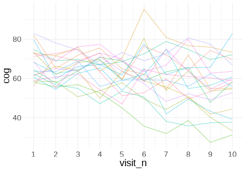
```

![](02_intromlm_files/figure-html/unnamed-chunk-38-1.png)
]

---
# MLM Example

__determining our random effect structure__

- multiple data-points per participant: **1 | participant**

- explanatory variable of interest (`visit_n`) varies *within* participants: **visit_n | participant**

- allow by-participant intercepts to correlate with by-participant slopes: **1 + visit_n | participant**  
(more on this in future weeks)

__fitting the model__

```r
cogtime_model <- lmer(cog ~ visit_n + (1 + visit_n | participant), data = cogtime)
```

---
# MLM Example

.pull-left[
__model output__

```r
summary(cogtime_model)
```

```
## Linear mixed model fit by REML ['lmerMod']
## Formula: cog ~ visit_n + (1 + visit_n | participant)
##    Data: cogtime
## 
## REML criterion at convergence: 1357
## 
## Scaled residuals: 
##    Min     1Q Median     3Q    Max 
## -2.274 -0.663 -0.091  0.577  3.227 
## 
## Random effects:
##  Groups      Name        Variance Std.Dev. Corr
##  participant (Intercept) 10.06    3.17         
##              visit_n      1.22    1.11     0.69
##  Residual                37.93    6.16         
## Number of obs: 200, groups:  participant, 20
## 
## Fixed effects:
##             Estimate Std. Error t value
## (Intercept)    68.56       1.18    58.2
## visit_n        -1.22       0.29    -4.2
## 
## Correlation of Fixed Effects:
##         (Intr)
## visit_n -0.019
```
]
.pull-right[
__raw data__

```r
ggplot(cogtime, aes(x=visit_n, y = cog, col=participant))+
  geom_path(alpha = 0.5)+
  guides(col=FALSE)+
  scale_x_continuous(breaks=1:10)+
  themedapr3()
```

![](02_intromlm_files/figure-html/unnamed-chunk-41-1.png)
]

---
# MLM Example: Plotting the model
#### **sjPlot::plot_model()**

.pull-left[

```r
library(sjPlot)
plot_model(cogtime_model, type="pred")
```
]

--
.pull-right[

```
## $visit_n
```

![](02_intromlm_files/figure-html/unnamed-chunk-43-1.png)
]

---
# MLM Example: Plotting the model
#### **effects::effect()**

.pull-left[

```r
library(effects)
as.data.frame(effect("visit_n",cogtime_model))
```

```
##   visit_n   fit    se lower upper
## 1       1 67.34 1.208 64.96 69.72
## 2       3 64.90 1.452 62.04 67.77
## 3       6 61.25 2.083 57.14 65.35
## 4       8 58.81 2.582 53.72 63.90
## 5      10 56.37 3.110 50.24 62.50
```

```r
as.data.frame(effect("visit_n",cogtime_model)) %>%
  ggplot(.,aes(x=visit_n, y=fit))+
  geom_line()+
  geom_ribbon(aes(ymin=lower,ymax=upper), alpha=.3)+
  themedapr3()
```
]

.pull-right[
![](02_intromlm_files/figure-html/unnamed-chunk-46-1.png)
]

---
# MLM Example: Plotting the model
#### **broom.mixed::augment()** for cluster-specific fits

.pull-left[

```r
library(broom.mixed)
augment(cogtime_model)
```

```
## # A tibble: 200 × 14
##      cog visit_n participant .fitted  .resid   .hat  .cooksd .fixed   .mu .offset
##    <dbl>   <dbl> <fct>         <dbl>   <dbl>  <dbl>    <dbl>  <dbl> <dbl>   <dbl>
##  1  56.1       1 1              69.7 -13.6   0.0782 0.225      67.3  69.7       0
##  2  71.5       2 1              69.6   1.93  0.0684 0.00386    66.1  69.6       0
##  3  68.9       3 1              69.5  -0.611 0.0653 0.000369   64.9  69.5       0
##  4  73.0       4 1              69.3   3.62  0.0690 0.0138     63.7  69.3       0
##  5  59.4       5 1              69.2  -9.79  0.0793 0.118      62.5  69.2       0
##  6  76.4       6 1              69.1   7.32  0.0964 0.0833     61.2  69.1       0
##  7  72.1       7 1              69.0   3.16  0.120  0.0204     60.0  69.0       0
##  8  64.2       8 1              68.8  -4.64  0.151  0.0594     58.8  68.8       0
##  9  74.3       9 1              68.7   5.65  0.188  0.120      57.6  68.7       0
## 10  69.7      10 1              68.6   1.16  0.232  0.00695    56.4  68.6       0
## # … with 190 more rows, and 4 more variables: .sqrtXwt <dbl>, .sqrtrwt <dbl>,
## #   .weights <dbl>, .wtres <dbl>
```

```r
ggplot(augment(cogtime_model), 
       aes(x=visit_n, y=.fitted,
           col=participant))+
  geom_line() +
  guides(col=FALSE)+
  themedapr3()
```
]

.pull-right[
![](02_intromlm_files/figure-html/unnamed-chunk-49-1.png)
]

---
# MLM Example: Tables

```r
library(sjPlot)
tab_model(cogtime_model)
```

<table style="border-collapse:collapse; border:none;">
<tr>
<th style="border-top: double; text-align:center; font-style:normal; font-weight:bold; padding:0.2cm;  text-align:left; ">&nbsp;</th>
<th colspan="3" style="border-top: double; text-align:center; font-style:normal; font-weight:bold; padding:0.2cm; ">cog</th>
</tr>
<tr>
<td style=" text-align:center; border-bottom:1px solid; font-style:italic; font-weight:normal;  text-align:left; ">Predictors</td>
<td style=" text-align:center; border-bottom:1px solid; font-style:italic; font-weight:normal;  ">Estimates</td>
<td style=" text-align:center; border-bottom:1px solid; font-style:italic; font-weight:normal;  ">CI</td>
<td style=" text-align:center; border-bottom:1px solid; font-style:italic; font-weight:normal;  ">p</td>
</tr>
<tr>
<td style=" padding:0.2cm; text-align:left; vertical-align:top; text-align:left; ">(Intercept)</td>
<td style=" padding:0.2cm; text-align:left; vertical-align:top; text-align:center;  ">68.56</td>
<td style=" padding:0.2cm; text-align:left; vertical-align:top; text-align:center;  ">66.25&nbsp;&ndash;&nbsp;70.87</td>
<td style=" padding:0.2cm; text-align:left; vertical-align:top; text-align:center;  "><strong>&lt;0.001</strong></td>
</tr>
<tr>
<td style=" padding:0.2cm; text-align:left; vertical-align:top; text-align:left; ">visit_n</td>
<td style=" padding:0.2cm; text-align:left; vertical-align:top; text-align:center;  ">&#45;1.22</td>
<td style=" padding:0.2cm; text-align:left; vertical-align:top; text-align:center;  ">&#45;1.79&nbsp;&ndash;&nbsp;-0.65</td>
<td style=" padding:0.2cm; text-align:left; vertical-align:top; text-align:center;  "><strong>&lt;0.001</strong></td>
</tr>
<tr>
<td colspan="4" style="font-weight:bold; text-align:left; padding-top:.8em;">Random Effects</td>
</tr>

<tr>
<td style=" padding:0.2cm; text-align:left; vertical-align:top; text-align:left; padding-top:0.1cm; padding-bottom:0.1cm;">&sigma;<sup>2</sup></td>
<td style=" padding:0.2cm; text-align:left; vertical-align:top; padding-top:0.1cm; padding-bottom:0.1cm; text-align:left;" colspan="3">37.93</td>

<tr>
<td style=" padding:0.2cm; text-align:left; vertical-align:top; text-align:left; padding-top:0.1cm; padding-bottom:0.1cm;">&tau;<sub>00</sub> <sub>participant</sub></td>
<td style=" padding:0.2cm; text-align:left; vertical-align:top; padding-top:0.1cm; padding-bottom:0.1cm; text-align:left;" colspan="3">10.06</td>

<tr>
<td style=" padding:0.2cm; text-align:left; vertical-align:top; text-align:left; padding-top:0.1cm; padding-bottom:0.1cm;">&tau;<sub>11</sub> <sub>participant.visit_n</sub></td>
<td style=" padding:0.2cm; text-align:left; vertical-align:top; padding-top:0.1cm; padding-bottom:0.1cm; text-align:left;" colspan="3">1.22</td>

<tr>
<td style=" padding:0.2cm; text-align:left; vertical-align:top; text-align:left; padding-top:0.1cm; padding-bottom:0.1cm;">&rho;<sub>01</sub> <sub>participant</sub></td>
<td style=" padding:0.2cm; text-align:left; vertical-align:top; padding-top:0.1cm; padding-bottom:0.1cm; text-align:left;" colspan="3">0.69</td>

<tr>
<td style=" padding:0.2cm; text-align:left; vertical-align:top; text-align:left; padding-top:0.1cm; padding-bottom:0.1cm;">N <sub>participant</sub></td>
<td style=" padding:0.2cm; text-align:left; vertical-align:top; padding-top:0.1cm; padding-bottom:0.1cm; text-align:left;" colspan="3">20</td>
<tr>
<td style=" padding:0.2cm; text-align:left; vertical-align:top; text-align:left; padding-top:0.1cm; padding-bottom:0.1cm; border-top:1px solid;">Observations</td>
<td style=" padding:0.2cm; text-align:left; vertical-align:top; padding-top:0.1cm; padding-bottom:0.1cm; text-align:left; border-top:1px solid;" colspan="3">200</td>
</tr>
<tr>
<td style=" padding:0.2cm; text-align:left; vertical-align:top; text-align:left; padding-top:0.1cm; padding-bottom:0.1cm;">Marginal R<sup>2</sup> / Conditional R<sup>2</sup></td>
<td style=" padding:0.2cm; text-align:left; vertical-align:top; padding-top:0.1cm; padding-bottom:0.1cm; text-align:left;" colspan="3">0.092 / 0.717</td>
</tr>

</table>

---
# Summary

- We can extend our linear model equation to model certain parameters as random cluster-level adjustments around a fixed center.

- `$\color{red}{y_i} = \color{blue}{\beta_0 \cdot{} 1 \; + \; \beta_1 \cdot{} x_{i} } + \varepsilon_i$`  
becomes  
`$\color{red}{y_{ij}} = \color{blue}{\beta_{0i} \cdot 1 + \beta_{1i} \cdot x_{ij}} + \varepsilon_{ij}$`  
`$\color{blue}{\beta_{0i}} = \gamma_{00} + \color{orange}{\zeta_{0i}}$`

- We can express this as one equation if we prefer:
`$\color{red}{y_{ij}} = \underbrace{(\gamma_{00} + \color{orange}{\zeta_{0i}})}_{\color{blue}{\beta_{0i}}} \cdot 1 +  \color{blue}{\beta_{1i} \cdot x_{ij}}  +  \varepsilon_{ij}$`

- This allows us to model cluster-level variation around the intercept ("random intercept") and around slopes ("random slope").

- We can fit this using the **lme4** package in R

---
class: inverse, center, middle, animated, rotateInDownLeft

# End of Part 1

---
class: inverse, center, middle

<h2 style="text-align: left;opacity:0.3;">Part 1: LM to MLM</h2>
<h2>Part 2: Inference in MLM</h2>

---
# <p></p>

.pull-left[
you might have noticed...

```r
summary(cogtime_model)
```

```
## Linear mixed model fit by REML ['lmerMod']
## Formula: cog ~ visit_n + (1 + visit_n | participant)
##    Data: cogtime
## 
## REML criterion at convergence: 1357
## 
## Scaled residuals: 
##    Min     1Q Median     3Q    Max 
## -2.274 -0.663 -0.091  0.577  3.227 
## 
## Random effects:
##  Groups      Name        Variance Std.Dev. Corr
##  participant (Intercept) 10.06    3.17         
##              visit_n      1.22    1.11     0.69
##  Residual                37.93    6.16         
## Number of obs: 200, groups:  participant, 20
## 
## Fixed effects:
##             Estimate Std. Error t value
*## (Intercept)    68.56       1.18    58.2
*## visit_n        -1.22       0.29    -4.2
## 
## Correlation of Fixed Effects:
##         (Intr)
## visit_n -0.019
```
]
.pull-right[
![](jk_img_sandbox/wotnop.png)
]

---
# Why no p-values?

**Extensive debate about how best to test parameters from MLMs.**

In simple LM, we test the reduction in residual SS (sums of squares), which follows an `$F$` distribution with a known `$df$`.
$$
`\begin{align}
F \qquad = \qquad \frac{MS_{model}}{MS_{residual}} \qquad = \qquad \frac{SS_{model}/df_{model}}{SS_{residual}/df_{residual}} \\
\quad \\
df_{model} = k \\
df_{residual} = n-k-1 \\
\end{align}`
$$
--

The `$t$`-statistic for a coefficient in a simple regression model is the square root of `$F$` ratio between models with and without that parameter.

- Such `$F$` will have 1 numerator degree of freedom (and `$n-k-1$` denominator degrees of freedom).
- The analogous `$t$`-distribution has `$n-k-1$` degrees of freedom

---
# Why no p-values?

In MLM, the distribution of a test statistic when the null hypothesis is true is **unknown.**

Under very specific conditions (normally distributed outcome variable, perfectly balanced designs), we can use an `$F$` distribution and correctly determine the denominator `$df$`.

But for most situations:
  - unclear how to calculate denominator `$df$`
  - unclear whether the test statistics even follow an `$F$` distribution

---
# Options for inference

1. df approximations

2. Likelihood Ratio Tests

3. Bootstrap

---
count:false
class: extra
exclude: FALSE
# Satterthwaite df approximation

.pull-left[
- There are some suggested approaches to approximating the denominator `$df$`. 
<br><br>
- Loading the package **lmerTest** will fit your models and print the summary with p-values approximated by the Satterthwaite method.

```r
library(lmerTest)
full_model <- lmer(cog ~  1 + visit_n + (1 + visit_n | participant), data = cogtime)
summary(full_model)
```
]
.pull-right[

```
## Linear mixed model fit by REML. t-tests use Satterthwaite's method [
## lmerModLmerTest]
## Formula: cog ~ 1 + visit_n + (1 + visit_n | participant)
##    Data: cogtime
## 
## REML criterion at convergence: 1357
## 
## Scaled residuals: 
##    Min     1Q Median     3Q    Max 
## -2.274 -0.663 -0.091  0.577  3.227 
## 
## Random effects:
##  Groups      Name        Variance Std.Dev. Corr
##  participant (Intercept) 10.06    3.17         
##              visit_n      1.22    1.11     0.69
##  Residual                37.93    6.16         
## Number of obs: 200, groups:  participant, 20
## 
## Fixed effects:
##             Estimate Std. Error    df t value Pr(>|t|)    
## (Intercept)    68.56       1.18 19.00    58.2  < 2e-16 ***
## visit_n        -1.22       0.29 19.00    -4.2  0.00048 ***
## ---
## Signif. codes:  0 '***' 0.001 '**' 0.01 '*' 0.05 '.' 0.1 ' ' 1
## 
## Correlation of Fixed Effects:
##         (Intr)
## visit_n -0.019
```
]

---
count:false
class: extra
exclude: FALSE
# Kenward-Rogers df approximations

- The **pbkrtest** package implements the slightly more reliable Kenward-Rogers method.

```r
library(pbkrtest)
restricted_model <- lmer(cog ~ 1 + (1 + visit_n | participant), data = cogtime)
full_model <- lmer(cog ~ 1 + visit_n + (1 + visit_n | participant), data = cogtime)
KRmodcomp(full_model, restricted_model)
```

```
## large : cog ~ 1 + visit_n + (1 + visit_n | participant)
## small : cog ~ 1 + (1 + visit_n | participant)
##       stat  ndf  ddf F.scaling p.value    
## Ftest 17.7  1.0 19.0         1 0.00048 ***
## ---
## Signif. codes:  0 '***' 0.001 '**' 0.01 '*' 0.05 '.' 0.1 ' ' 1
```

---
count:false
class: extra
exclude: FALSE
# Likelihood ratio tests

.pull-left[
We can also conduct a Likelihood Ratio Test (LRT).

```r
anova(restricted_model, full_model, test = "LRT")
```

```
## Data: cogtime
## Models:
## restricted_model: cog ~ 1 + (1 + visit_n | participant)
## full_model: cog ~ 1 + visit_n + (1 + visit_n | participant)
##                  npar  AIC  BIC logLik deviance Chisq Df Pr(>Chisq)    
## restricted_model    5 1382 1398   -686     1372                        
## full_model          6 1370 1390   -679     1358  13.2  1    0.00029 ***
## ---
## Signif. codes:  0 '***' 0.001 '**' 0.01 '*' 0.05 '.' 0.1 ' ' 1
```

]

.pull-right[
- Compares the log-likelihood of two competing models.  
<br><br>
- what is the "likelihood"?  
    - a function that associates to a parameter the probability (or probability density) of observing the given sample data. 
<br><br>
- ratio of two likelihoods is asymptotically `$\chi^2$`-square distributed.
    - **this means for small samples it may be unreliable**
]

---
# Options for inference

1. <p style="opacity:.4"> df approximations - assumes `$F$`-distributed just with unknown `$ddf$`.<p>

2. <p style="opacity:.4">Likelihood Ratio Tests - differences in logLik are only asymptotically `$\chi^2$`distributed.</p>

3. Bootstrap  
  - Parametric Bootstrap  
  assumes that explanatory variables are fixed and that model specification and the distributions such as `$\zeta_i \sim N(0,\sigma_{\zeta})$` and `$\varepsilon_i \sim N(0,\sigma_{\varepsilon})$` are correct.
  
  - Case-based Bootstrap  
  minimal assumptions - we just need to ensure that we correctly specify the hierarchical dependency of data.  
  requires decision of at which levels to resample.  
  (discussed more next week)

---
# Parametric Bootstrap

.pull-left[
The idea here is that in order to do inference on the effect of a (set of) predictor(s), you

1. fit the reduced model (without the predictors) to the data. 
{{content}}
]

2. Do many times:  
  - simulate data from the reduced model
  - fit both the reduced and the full model to the simulated (null) data
  - compute some statistic(s), e.g. likelihood ratio.
{{content}}

3. Compare the parameter estimates obtained from fitting models to the **data**, to the "null distribution" constructed in step 2.

.pull-right[
Easy to do with `PBmodcomp()` in the **pbkrtest** package.

```r
library(pbkrtest)
PBmodcomp(full_model, restricted_model)
```

```
## Bootstrap test; time: 27.43 sec; samples: 1000; extremes: 1;
## Requested samples: 1000 Used samples: 989 Extremes: 1
## large : cog ~ 1 + visit_n + (1 + visit_n | participant)
## cog ~ 1 + (1 + visit_n | participant)
##        stat df p.value    
## LRT    13.1  1 0.00029 ***
## PBtest 13.1    0.00202 ** 
## ---
## Signif. codes:  0 '***' 0.001 '**' 0.01 '*' 0.05 '.' 0.1 ' ' 1
```
]

---
# Summary

- Lots of debate around how best to conduct statistical inferences based on multi-level models. 
  - denominator degrees of freedom can't be calculated, so traditional `$F$` tests cannot be conducted

- Lots of other options (approximations for `$df$`, likelihood ratio tests, bootstrap)
  - The choice is yours, but we recommend bootstrapping (of which there are also many different approaches!)

---
count:false
class: center, middle, animated, rotateInDownLeft

<b style="opacity:0.4;">take a break... </b>

---
class: inverse, center, middle

<h2 style="text-align: left;opacity:0.3;">Part 1: LM to MLM</h2>
<h2><b style="opacity:0.4;">Part 2: Inference in MLM </b><b>Examples</b></h2>

---
# Data

```r
nursedf <- read_csv("https://uoepsy.github.io/data/nurse_stress.csv")
nursedf <- nursedf %>% 
  mutate(across(c(hospital, expcon, gender, wardtype, hospsize), factor))
head(nursedf)
```

```
## # A tibble: 6 × 10
##   hospital expcon nurse   age gender experien stress Zstress wardtype   hospsize
##   <fct>    <fct>  <dbl> <dbl> <fct>     <dbl>  <dbl>   <dbl> <fct>      <fct>   
## 1 1        1          1    36 0            11      7    2.07 general c… large   
## 2 1        1          2    45 0            20      7    2.07 general c… large   
## 3 1        1          3    32 0             7      7    2.07 general c… large   
## 4 1        1          4    57 1            25      6    1.04 general c… large   
## 5 1        1          5    46 1            22      6    1.04 general c… large   
## 6 1        1          6    60 1            22      6    1.04 general c… large
```

_The files nurses.csv contains three-level simulated data from a hypothetical study on stress in hospitals. The data are from nurses working in wards nested within hospitals. It is a cluster-randomized experiment. In each of 25 hospitals, four wards are selected and randomly assigned to an experimental and a control condition. In the experimental condition, a training program is offered to all nurses to cope with job-related stress. After the program is completed, a sample of about 10 nurses from each ward is given a test that measures job-related stress. Additional variables are: nurse age (years), nurse experience (years), nurse gender (0 = male, 1 = female), type of ward (0 = general care, 1 = special care), and hospital size (0 = small, 1 = medium, 2 = large)._  
(From https://multilevel-analysis.sites.uu.nl/datasets/ )

---
# test of a single parameter

> After accounting for nurses' age, gender and experience, does having been offered a training program to cope with job-related stress appear to reduce levels of stress, and if so, by how much?

```r
mod1 <- lmer(Zstress ~ 1 + experien + age + gender + expcon + (1 | hospital), data = nursedf)
summary(mod1)
```

```
## Linear mixed model fit by REML ['lmerMod']
## Formula: Zstress ~ 1 + experien + age + gender + expcon + (1 | hospital)
##    Data: nursedf
## 
## REML criterion at convergence: 2218
## 
## Scaled residuals: 
##    Min     1Q Median     3Q    Max 
## -2.950 -0.672  0.026  0.645  3.192 
## 
## Random effects:
##  Groups   Name        Variance Std.Dev.
##  hospital (Intercept) 0.296    0.544   
##  Residual             0.484    0.696   
## Number of obs: 1000, groups:  hospital, 25
## 
## Fixed effects:
##             Estimate Std. Error t value
## (Intercept)  0.90568    0.14386    6.30
## experien    -0.05912    0.00638   -9.26
## age          0.01965    0.00320    6.15
## gender1     -0.46214    0.05045   -9.16
## expcon1     -0.76007    0.04403  -17.26
## 
## Correlation of Fixed Effects:
##          (Intr) expern age    gendr1
## experien  0.018                     
## age      -0.338 -0.817              
## gender1  -0.269  0.026 -0.006       
## expcon1  -0.165  0.000  0.015 -0.015
```

---
count:false
class: extra
exclude: FALSE
# test of a single parameter

> After accounting for nurses' age, gender and experience, does having been offered a training program to cope with job-related stress appear to reduce levels of stress, and if so, by how much?

__Likelihood Ratio Test:__

```r
mod0 <- lmer(Zstress ~ 1 + experien + age + gender + (1 | hospital), data = nursedf)
mod1 <- lmer(Zstress ~ 1 + experien + age + gender + expcon + (1 | hospital), data = nursedf)
anova(mod0, mod1, test="Chisq")
```

```
## Data: nursedf
## Models:
## mod0: Zstress ~ 1 + experien + age + gender + (1 | hospital)
## mod1: Zstress ~ 1 + experien + age + gender + expcon + (1 | hospital)
##      npar  AIC  BIC logLik deviance Chisq Df Pr(>Chisq)    
## mod0    6 2461 2490  -1224     2449                        
## mod1    7 2202 2236  -1094     2188   261  1     <2e-16 ***
## ---
## Signif. codes:  0 '***' 0.001 '**' 0.01 '*' 0.05 '.' 0.1 ' ' 1
```

---
count:false
# test of a single parameter

> After accounting for nurses' age, gender and experience, does having been offered a training program to cope with job-related stress appear to reduce levels of stress, and if so, by how much?

__Parametric Bootstrap__

```r
mod0 <- lmer(Zstress ~ 1 + experien + age + gender + (1 | hospital), data = nursedf)
mod1 <- lmer(Zstress ~ 1 + experien + age + gender +  expcon + (1 | hospital), data = nursedf)
PBmodcomp(mod1, mod0)
```

```
## Bootstrap test; time: 23.01 sec; samples: 1000; extremes: 0;
## large : Zstress ~ 1 + experien + age + gender + expcon + (1 | hospital)
## Zstress ~ 1 + experien + age + gender + (1 | hospital)
##        stat df p.value    
## LRT     261  1  <2e-16 ***
## PBtest  261      0.001 ***
## ---
## Signif. codes:  0 '***' 0.001 '**' 0.01 '*' 0.05 '.' 0.1 ' ' 1
```

---
count:false
# test of a single parameter

> After accounting for nurses' age, gender and experience, does having been offered a training program to cope with job-related stress appear to reduce levels of stress, and if so, **by how much?**

__Parametric Bootstrap Confidence Intervals__

```r
mod1 <- lmer(Zstress ~ 1 + experien + age + gender +  expcon + (1 | hospital), data = nursedf)
confint(mod1, method="boot")
```

```
##                2.5 %   97.5 %
## .sig01       0.39476  0.70600
## .sigma       0.66009  0.72655
## (Intercept)  0.61711  1.18782
## experien    -0.07269 -0.04748
## age          0.01368  0.02616
## gender1     -0.55448 -0.36142
*## expcon1     -0.83685 -0.67703
```

---
count:false
# test of a single parameter

> After accounting for nurses' age, gender and experience, does having been offered a training program to cope with job-related stress appear to reduce levels of stress, and if so, by how much?

Attendance of training programs on job-related stress was found to predict stress levels of nurses in 25 hospitals, beyond individual nurses' years of experience, age and gender (Parametric Bootstrap Likelihood Ratio Test statistic = 260.919, p<.001). Having attended the training program was associated with a decrease in -0.7601 (Bootstrap 95% CI [-0.84, -0.68] ) standard deviations on the measure of job-related stress.

---
count:false
class: extra
exclude: FALSE
# testing that several parameters are simultaneously zero

> Do ward type and hospital size influence levels of stress in nurses beyond the effects of age, gender, training and experience?

__Likelihood Ratio Test__

```r
mod0 <- lmer(Zstress ~ experien + age + gender + expcon + (1 | hospital), data = nursedf)
mod1 <- lmer(Zstress ~ experien + age + gender + expcon + wardtype + hospsize + (1 | hospital), data = nursedf)
anova(mod0, mod1, test="Chisq")
```

```
## Data: nursedf
## Models:
## mod0: Zstress ~ experien + age + gender + expcon + (1 | hospital)
## mod1: Zstress ~ experien + age + gender + expcon + wardtype + hospsize + (1 | hospital)
##      npar  AIC  BIC logLik deviance Chisq Df Pr(>Chisq)   
## mod0    7 2202 2236  -1094     2188                       
## mod1   10 2194 2243  -1087     2174    14  3     0.0029 **
## ---
## Signif. codes:  0 '***' 0.001 '**' 0.01 '*' 0.05 '.' 0.1 ' ' 1
```

---
count:false
class: extra
exclude: FALSE
# testing that several parameters are simultaneously zero

> Do ward type and hospital size influence levels of stress in nurses beyond the effects of age, gender, training and experience?

__Kenward-Rogers `$df$`-approximation__

```
## large : Zstress ~ experien + age + gender + expcon + wardtype + hospsize + 
##     (1 | hospital)
## small : Zstress ~ experien + age + gender + expcon + (1 | hospital)
##        stat   ndf   ddf F.scaling p.value   
## Ftest  4.99  3.00 40.27     0.988  0.0049 **
## ---
## Signif. codes:  0 '***' 0.001 '**' 0.01 '*' 0.05 '.' 0.1 ' ' 1
```

---
# testing that several parameters are simultaneously zero

> Do ward type and hospital size influence levels of stress in nurses beyond the effects of age, gender, training and experience?

__Parametric Bootstrap__

```
## Bootstrap test; time: 22.05 sec; samples: 1000; extremes: 3;
## large : Zstress ~ experien + age + gender + expcon + wardtype + hospsize + 
##     (1 | hospital)
## Zstress ~ experien + age + gender + expcon + (1 | hospital)
##        stat df p.value   
## LRT    13.8  3  0.0032 **
## PBtest 13.8     0.0040 **
## ---
## Signif. codes:  0 '***' 0.001 '**' 0.01 '*' 0.05 '.' 0.1 ' ' 1
```

---
# testing random effects

__are you sure you want to?__

- Justify the random effect structure based on study design, theory, and practicalities more than tests of significance.

- If needed, the __RLRsim__ package can test a single random effect (e.g. `lm()` vs `lmer()`).

```r
library(RLRsim)
mod0 <- lm(stress ~ expcon + experien + age + gender + wardtype + hospsize, data = nursedf)
mod1 <- lmer(stress ~ expcon + experien + age + gender + wardtype + hospsize + 
               (1 | hospital), data = nursedf)
exactLRT(m = mod1, m0 = mod0)
```

```
## 
## 	simulated finite sample distribution of LRT. (p-value based on 10000
## 	simulated values)
## 
## data:  
## LRT = 240, p-value <2e-16
```

---
class: inverse, center, middle, animated, rotateInDownLeft

# End