Categorical predictors and treatment coding


Data Analysis for Psychology in R 2

Dr. Elizabeth Pankratz (elizabeth.pankratz@ed.ac.uk)


Department of Psychology
University of Edinburgh
2026–2027

Course overview


Introduction to linear models
(with Dr. Patrick Sturt)
Introduction to linear regression
Interpreting linear models
Testing predictors and evaluating linear models
F-tests and model comparison
Practice analysis: Linear models
Extending linear models
(with Dr. Elizabeth Pankratz)
Categorical predictors and treatment coding
Sum coding
Assumptions and diagnostics
Bootstrapping and confidence intervals
Practice analysis: Categorical predictors (led by Patrick)
Interactions
(with Dr. Elizabeth Pankratz)
Mean-centering and numeric/categorical interactions
Numeric/numeric interactions
Categorical/categorical interactions
Testing simple effects and correcting for multiple comparisons
Practice analysis: Interactions (led by Patrick)
Logistic regression
(with Dr. Elizabeth Pankratz)
Probabilities and log-odds
Modelling binary outcomes with logistic regression
Interactions, assumptions, diagnostics, comparisons
Practice analysis: Logistic regression (led by Patrick)
Report feedback, exam prep, full-course Q&A

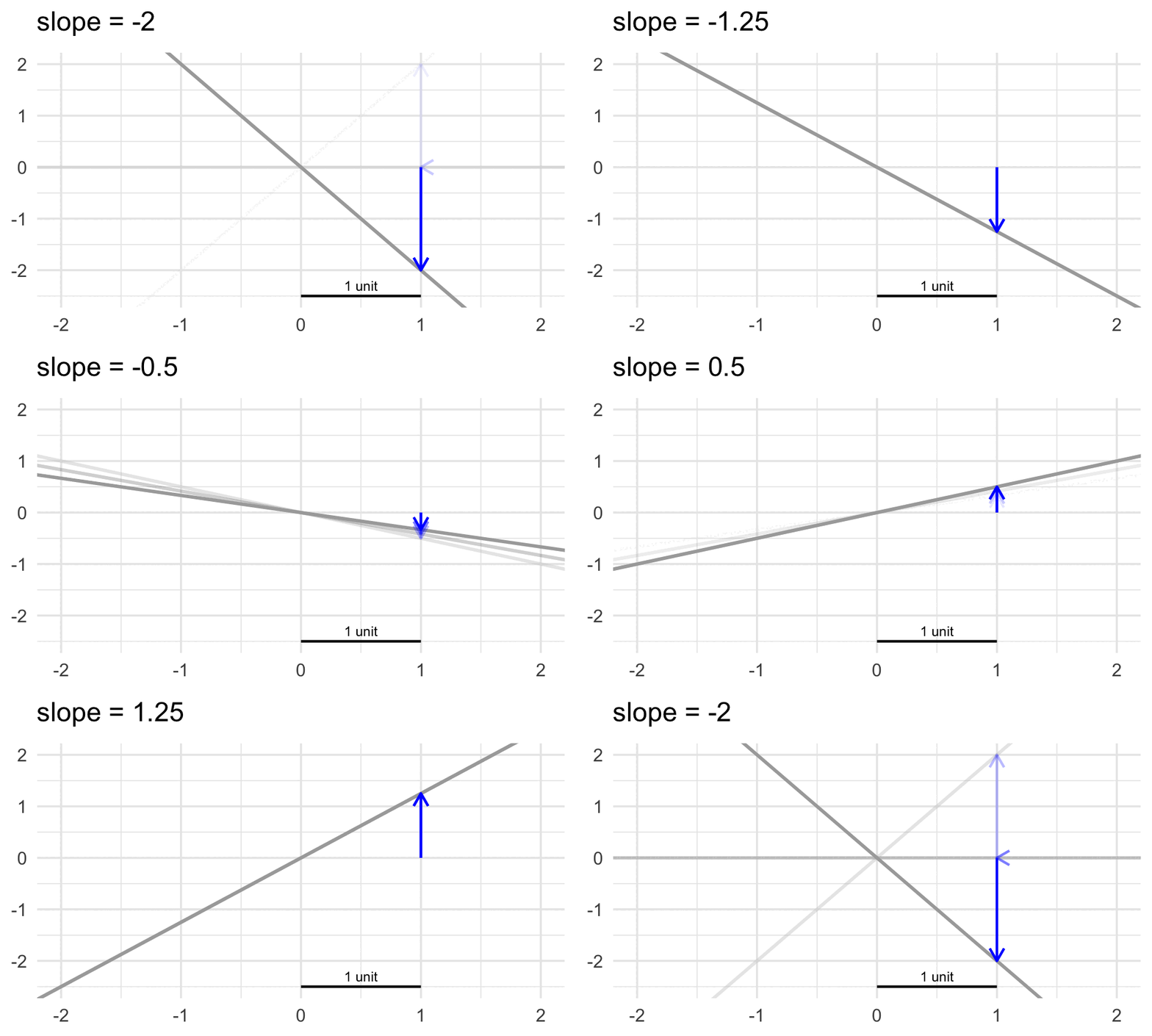
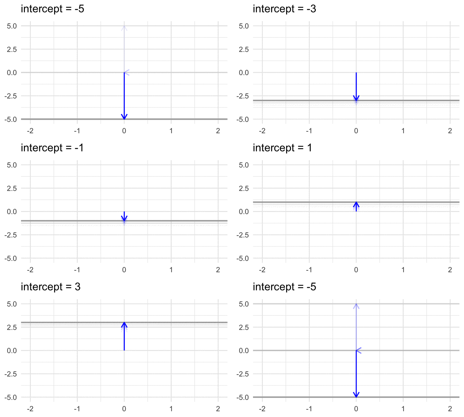
Warm-up: Think back to intercepts and slopes


What are intercepts? What are slopes?


A line’s intercept is its y-value (its outcome value) when x (the predictor) is 0.


A line’s slope is how much y (the outcome value) changes when x (the predictor) moves from 0 to 1.


This week’s learning objectives


How can we include categorical variables as predictors in a linear model?

When we use a categorical predictor, how do we interpret the linear model’s coefficients?

What hypotheses are tested by the default way that R represents categorical predictors?

What is “contrast coding”?

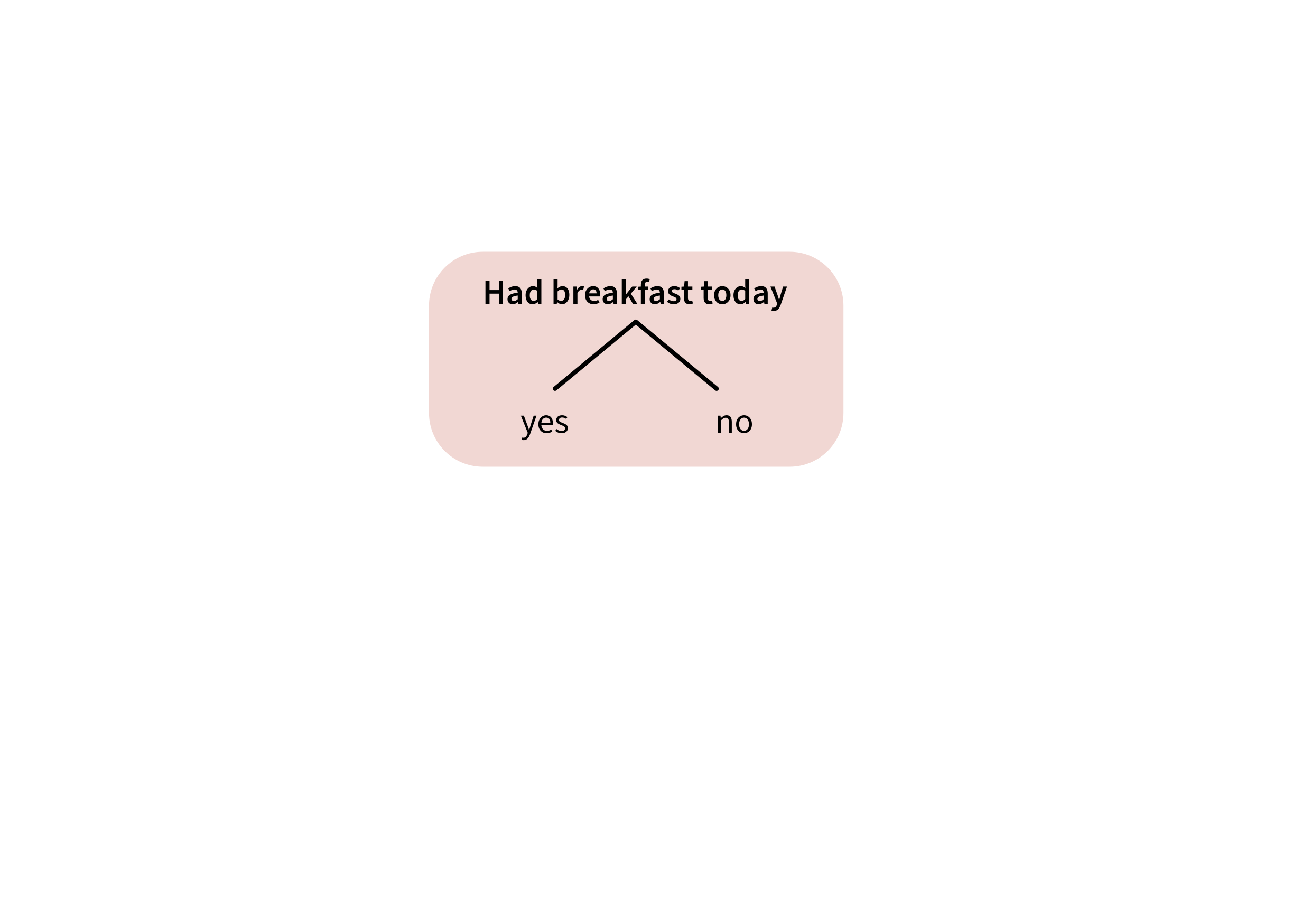
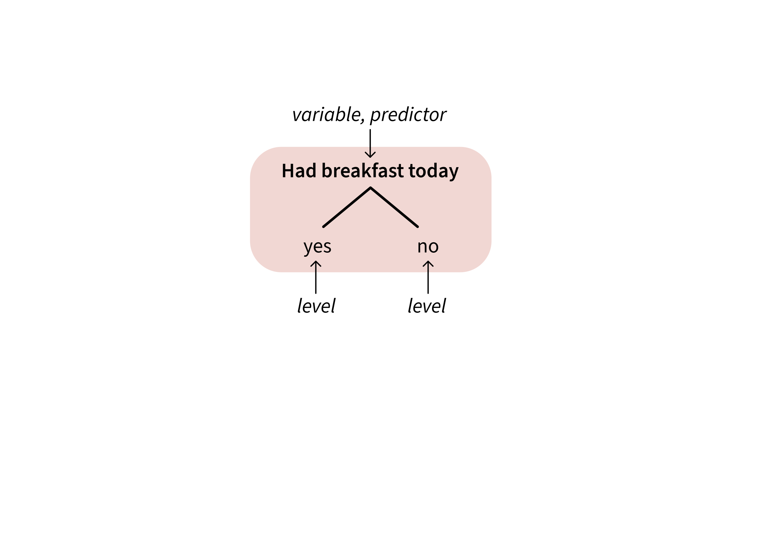
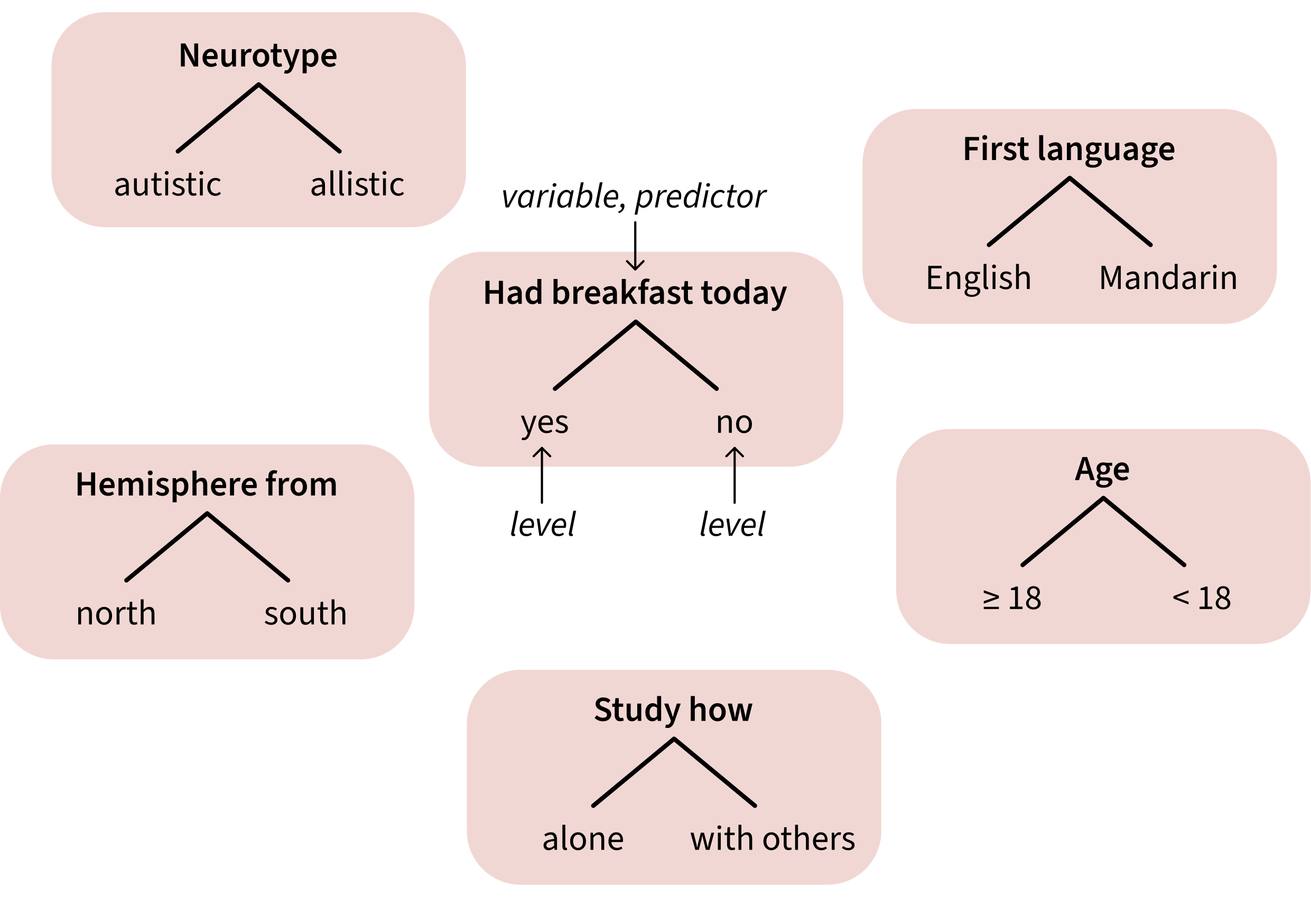
Categorical predictors with two levels

Categorical predictors with two levels,
aka binary predictors

Categorical predictors with two levels,
aka binary predictors

Categorical predictors with two levels,
aka binary predictors

But: linear models can only deal with input in number form.

So we need a way to represent the levels of these variables as numbers.

The way we’ll learn about today: treatment coding.

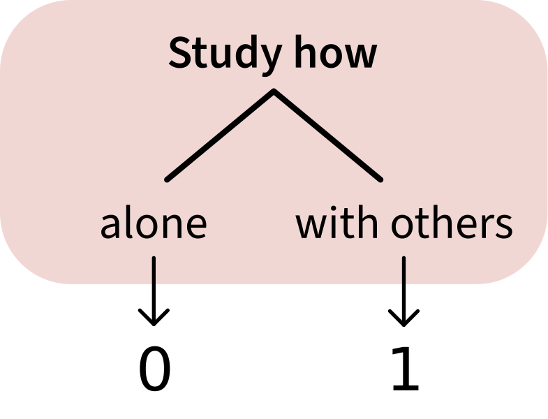
Treatment coding represents one level as 0,
and the other level as 1


The idea:

  • Studying alone is coded as 0.

  • Studying with others is coded as 1.

In the data:

score_data |>
  select(ID, study, study_num) |>
  head(10)
      ID  study study_num
1  ID101 others         1
2  ID102  alone         0
3  ID103  alone         0
4  ID104 others         1
5  ID105  alone         0
6  ID106 others         1
7  ID107  alone         0
8  ID108  alone         0
9  ID109 others         1
10 ID110  alone         0

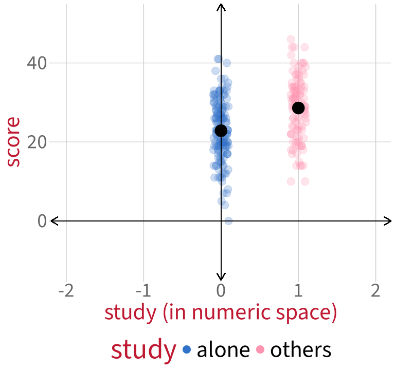
What does it mean to represent levels as 0 or 1?

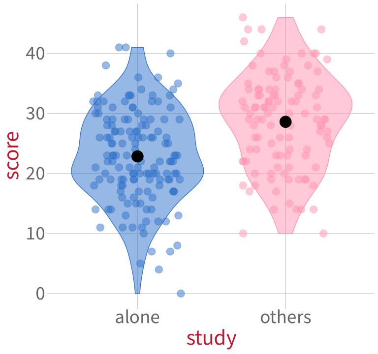
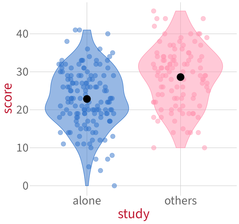
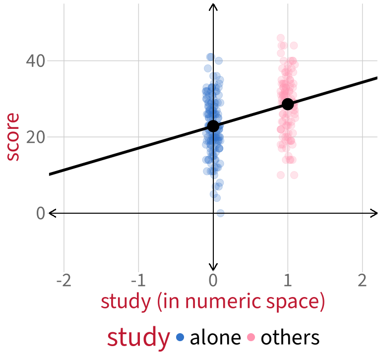
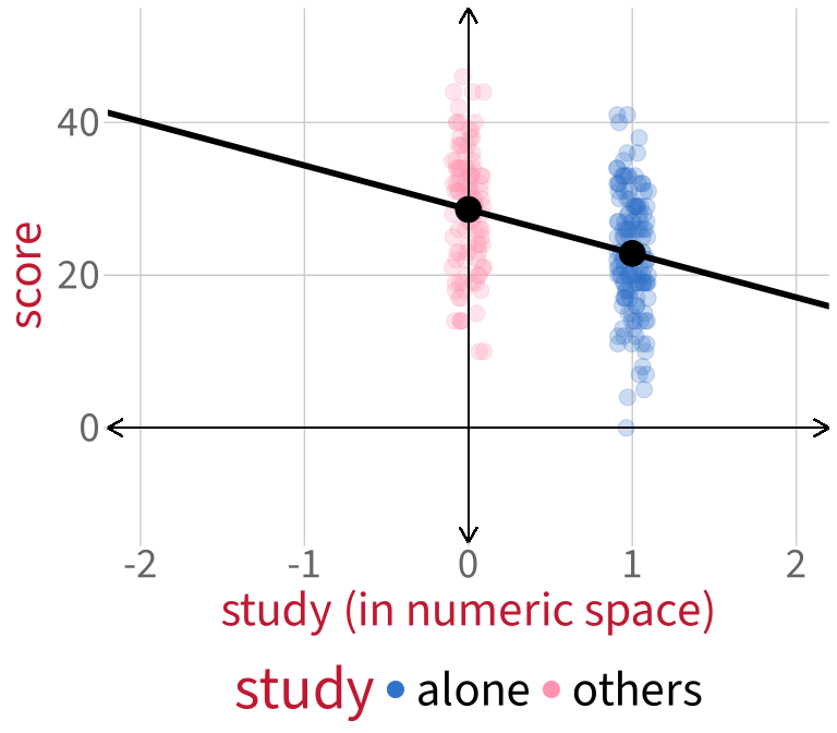
To illustrate: Here are test scores from students who studied either alone (blue) or with others (pink).

Code
set.seed(1)
p_viol_bin <- score_data |>
  ggplot(aes(x = study, y = score, fill = study, colour = study)) +
  geom_violin(alpha = 0.5) +
  geom_jitter(height = 0, alpha = 0.5, size = 5, width = 0.3) +
  theme(
    legend.position = 'none',
    panel.grid.minor = element_blank()
    ) +
  stat_summary(fun = mean, geom = 'point', colour = 'black', size = 8, show.legend = FALSE) +

  scale_colour_manual(values = pal) +
  scale_fill_manual(values = pal) +
  NULL
p_viol_bin

Code
xlim_lower <- -2.2
xlim_upper <-  2.2
ylim_lower <- -15
ylim_upper <-  55

set.seed(1)  # seed for constant jitter
p_xy_study <- score_data |>
  ggplot(aes(x = study_num, y = score)) +
  geom_jitter(aes(colour = study), height = 0, alpha = 0.25, width = 0.1, size = 5) +
  scale_x_continuous(limits = c(xlim_lower, xlim_upper), expand = c(0, 0)) +
  scale_y_continuous(limits = c(ylim_lower, ylim_upper), expand = c(0, 0)) +
  geom_segment(x = xlim_lower, xend = xlim_upper, y = 0, yend = 0,
               arrow = arrow(ends = 'both', length = unit(12, 'pt')), colour = 'black') +
  geom_segment(x = 0, xend = 0, y = ylim_lower, yend = ylim_upper, 
               arrow = arrow(ends = 'both', length = unit(12, 'pt')), colour = 'black') +
  stat_summary(fun = mean, geom = 'point', colour = 'black', size = 8, show.legend = FALSE) +

  scale_colour_manual(values = pal) +
  theme(
    panel.grid.minor = element_blank(),
    legend.position = 'bottom'
  ) +
  labs(
    x = 'study (in numeric space)'
  ) +
 guides(colour = guide_legend(override.aes = list(alpha = 1))) + 
  NULL

p_xy_study
What does it mean to represent levels as 0 or 1?

To illustrate: Here are test scores from students who studied either alone (blue) or with others (pink).

Code
set.seed(1)
p_viol_bin +
  # stat_summary(colour = 'black', fun = mean, geom = 'point', size = 2) +
  # geom_segment(aes(x = 'alone', xend = 'others', y = mean_alone, yend = mean_others), colour = 'black') +
  NULL

Code
set.seed(1)  # seed for constant jitter
p_xy_study <- p_xy_study +
  geom_abline(slope = mean_others - mean_alone, intercept = mean_alone, colour = 'black', linewidth = 2) +
  NULL
p_xy_study
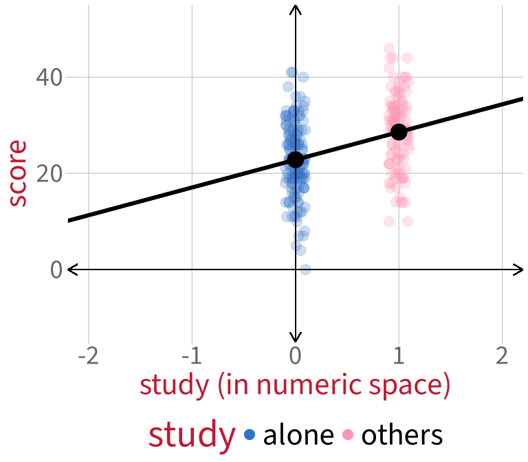
A linear model will fit a line to this data.

The line’s intercept will be the same as the mean of either alone or others. Which one? Why?

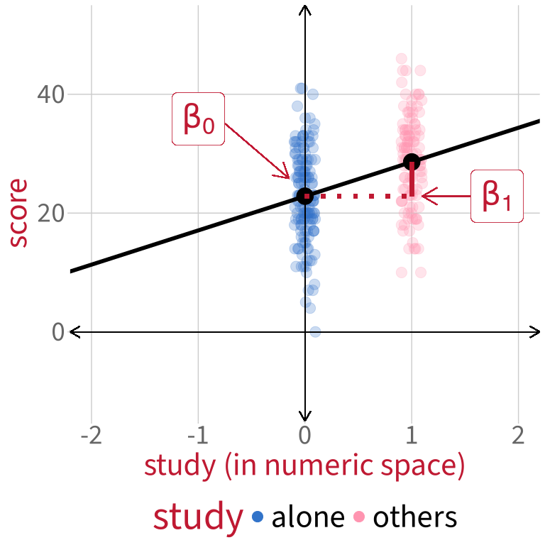
How do we describe this line?

Using our mathematical toolkit:

\[ \text{score} = \beta_0 + (\beta_1 \cdot \text{study}_{\text{others}}) + \epsilon \]


\(\beta_0\): intercept, mean of alone (the level represented as 0, which we call the reference level):

mean_alone
[1] 22.8


\(\beta_1\): slope, the difference between mean of others (represented as 1) and mean of alone (represented as 0):

mean_others - mean_alone
[1] 5.76


\(\epsilon\): error for each individual data point

Testing differences between levels

Testing differences between levels


We can find parameter values all on our own, without a linear model.

So why do we need to do statistical modelling?


Because what we can’t easily do by hand is statistically test research questions like:

Do students who study with others score significantly better than students who study alone?


To answer this question, we’ll fit a model that predicts score as a function of study patterns.

\[ \text{score} = \beta_0 + (\beta_1 \cdot \text{study}_\text{others}) + \epsilon \]


m1 <- lm(score ~ study, data = score_data)

Modelling score ~ study

summary(m1)

Call:
lm(formula = score ~ study, data = score_data)

Residuals:
    Min      1Q  Median      3Q     Max 
-22.846  -5.417   0.154   5.393  18.154 

Coefficients:
            Estimate Std. Error t value Pr(>|t|)    
(Intercept)   22.846      0.659   34.66  < 2e-16 ***
studyothers    5.761      1.008    5.72  3.1e-08 ***
---
Signif. codes:  0 '***' 0.001 '**' 0.01 '*' 0.05 '.' 0.1 ' ' 1

Residual standard error: 7.88 on 248 degrees of freedom
Multiple R-squared:  0.116, Adjusted R-squared:  0.113 
F-statistic: 32.7 on 1 and 248 DF,  p-value: 3.09e-08


Those coefficient estimates look familiar…

mean_alone
[1] 22.8
mean_others - mean_alone
[1] 5.76

Model evaluation works the same as before


\(R^2\):

  • Still tells us how much variance in the data is accounted for by the model.
Multiple R-squared:  0.116, Adjusted R-squared:  0.113 


\(F\)-ratio (aka \(F\)-statistic):

  • Still tells us the ratio of explained variance to unexplained variance.
  • Still tests the hypothesis that all regression slopes in the model = 0.
F-statistic: 32.7 on 1 and 248 DF,  p-value: 3.09e-08


(Revisit Lecture 4 for a refresher!)

What hypotheses are being tested for each coefficient? Same as always: that the estimate equals zero.

            Estimate Std. Error t value Pr(>|t|)
(Intercept)    22.85      0.659   34.66 4.76e-97
studyothers     5.76      1.008    5.72 3.09e-08


(Intercept) aka \(\beta_0\):

  • Null hypothesis (aka H0): the intercept is equal to zero (aka \(\beta_0 = 0\)).
  • \(p\)-value (aka Pr(>|t|)): the probability of observing an intercept of 22.85 (or even more extreme), assuming that the true value of the intercept is zero.

studyothers aka \(\beta_1\):

  • Null hypothesis (aka H0): the difference between levels is equal to zero (aka \(\beta_1 = 0\)).
  • \(p\)-value: the probability of observing a difference of 5.76 (or even more extreme), assuming that the true value of the difference is zero.


Our research question was about how studying alone or with others is associated with test score.

Are both of these hypothesis tests relevant to our research question?

Visualising the model’s predictions

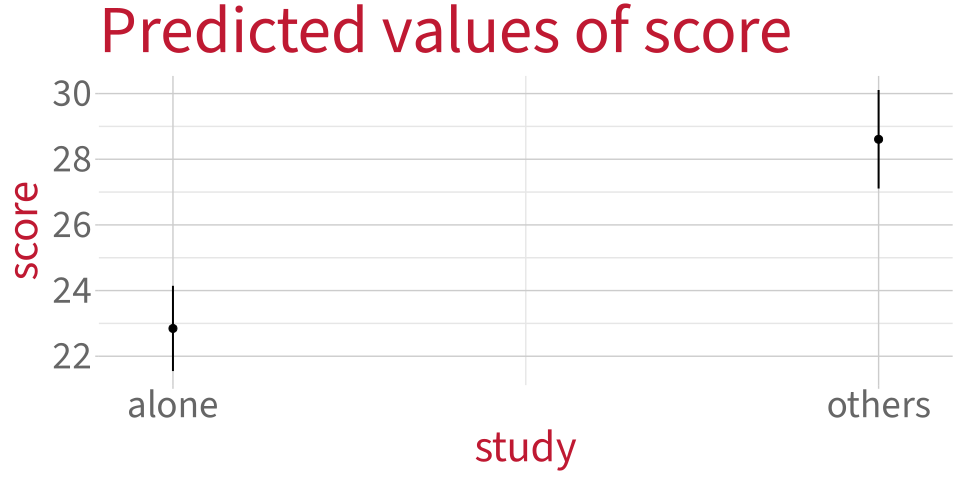
plot_model() from sjPlot works OK for categorical data too:

plot_model(
  m1,                # which model?
  type = 'eff',      # what kind of plot? (eff = "effect")
  terms = 'study',   # what predictor on x axis?
  colors = 'black'   # what colour to use?
)

Changing the reference level

Changing the reference level

If reference level = alone:

If reference level = others:

When others is the reference level (that is, the level represented as 0):

  • What does the intercept represent?
  • What does the slope represent?
  • Why is the slope negative now, when before it was positive?

How to change reference level in R?

The function contrasts() shows us how a categorical predictor will be coded. (You’ll get error messages if the variable is not stored as a factor.)

The original treatment coding:

contrasts(score_data$study)
       others
alone       0
others      1


Reorder factor levels in study, putting our desired reference level first:

score_data <- score_data |>
  mutate(
    study = factor(study, levels = c('others', 'alone'))
  )


Now check the contrasts. How can we tell that others is now the reference level?

contrasts(score_data$study)
       alone
others     0
alone      1

Fit a new model


Before:

\[ \text{score} = \beta_0 + (\beta_1 \cdot \text{study}_{\text{others}}) + \epsilon \]


Now:

\[ \text{score} = \beta_0 + (\beta_1 \cdot \text{study}_{\text{alone}}) + \epsilon \]


In R syntax, the model formula stays the same: score ~ study.

m2 <- lm(score ~ study, data = score_data)

Old model vs. new model


Reference level = alone (old model):

 Coefficients:
             Estimate Std. Error t value Pr(>|t|)    
 (Intercept)   22.846      0.659   34.66  < 2e-16 ***
 studyothers    5.761      1.008    5.72  3.1e-08 ***


Reference level = others (new model):

 Coefficients:
             Estimate Std. Error t value Pr(>|t|)    
 (Intercept)   28.607      0.762   37.54  < 2e-16 ***
 studyalone    -5.761      1.008   -5.72  3.1e-08 ***

How to choose appropriate reference level?


In treatment coding,

  • the intercept will always be the estimated mean outcome for the reference level (the level coded as 0).
  • the slope will always be the estimated difference between the non-reference level (coded as 1) and the reference level (coded as 0).

So how do you decide which level should be the reference level?


The most useful reference level is usually whatever the “control” group in your data is.

If there is no control group (like in this week’s examples), then the reference level can kind of be anything.

In future weeks, you’ll see examples of how the phrasing of a RQ can guide your choice of reference level.

What questions do you have right now?


Categorical predictors
with >2 levels

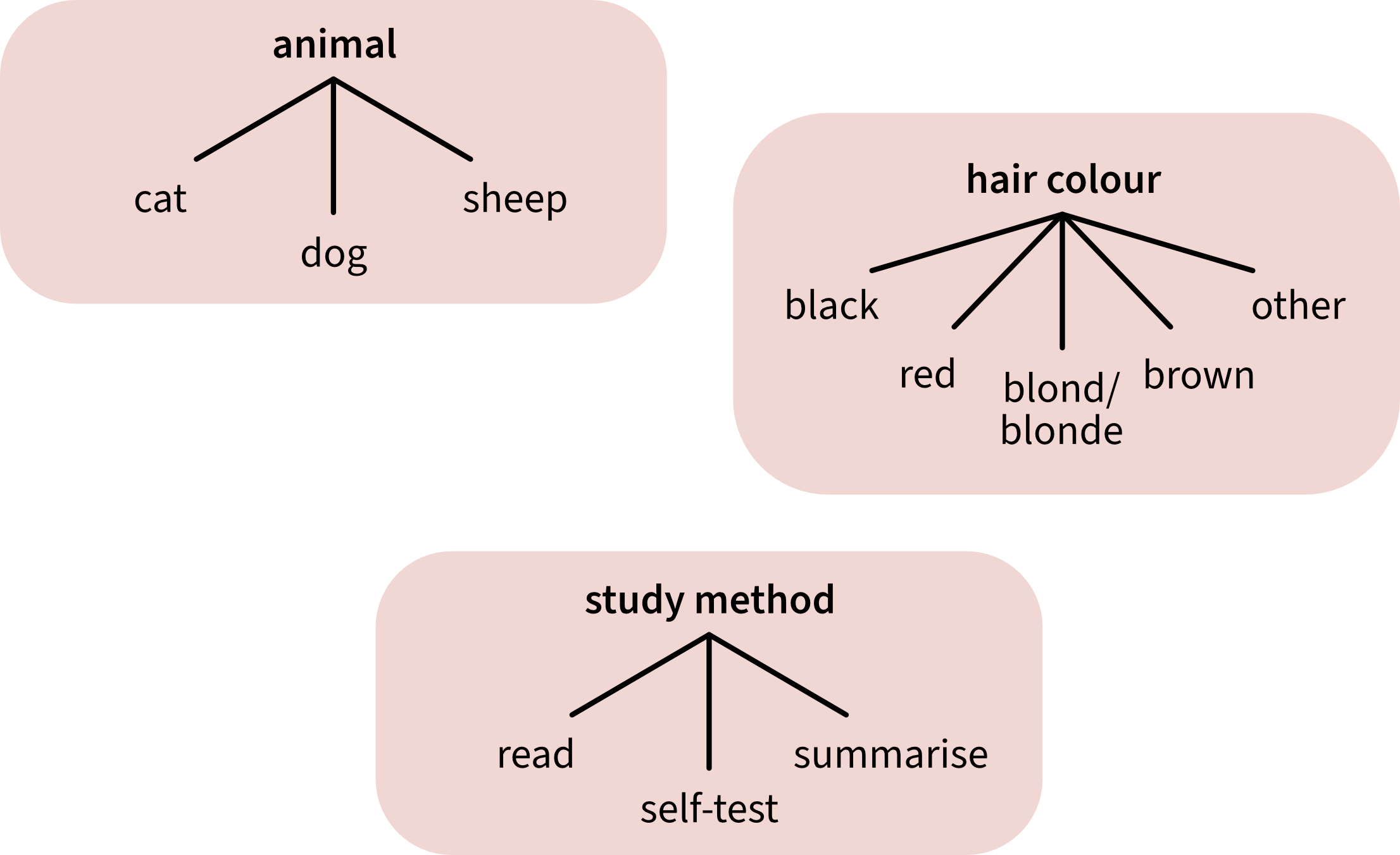
Examples of categorical predictors with >2 levels


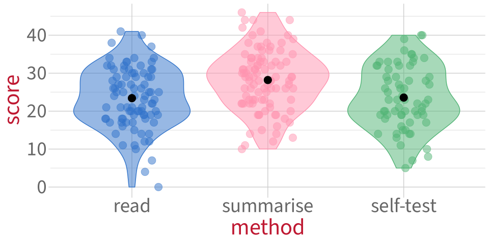
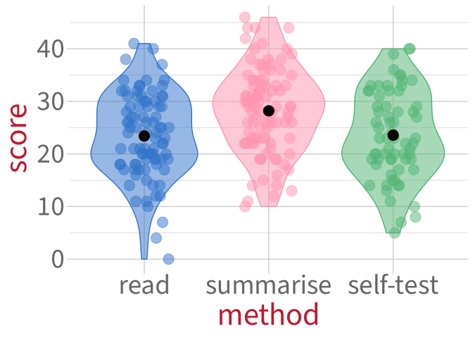
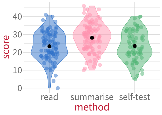
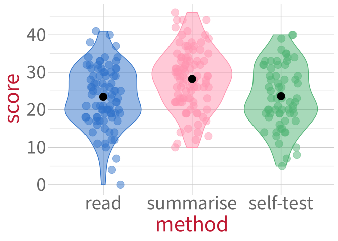
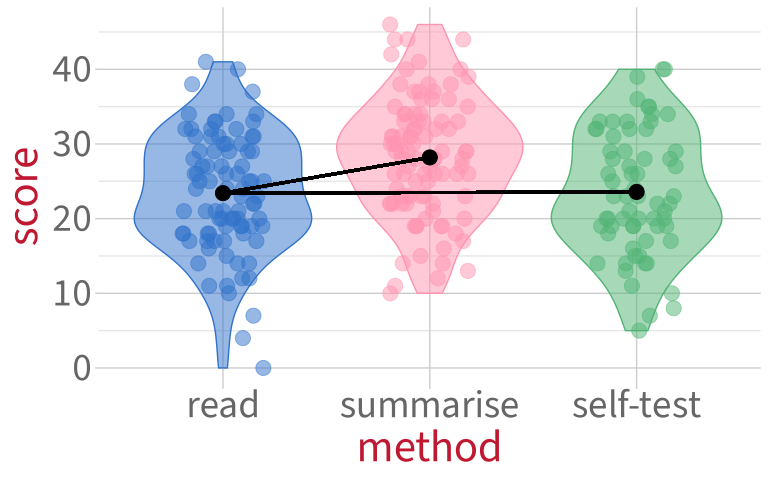
New data: Study method

Code
set.seed(1)
p_viol <- score_data |>
  ggplot(aes(x = method, y = score, fill = method, colour = method)) +
  geom_violin(alpha = 0.5) +
  geom_jitter(height = 0, alpha = 0.5, width = 0.2, size = 5) +
  theme(legend.position = 'none') +
  scale_fill_manual(values = pal) +
  scale_colour_manual(values = pal) +
  stat_summary(fun = mean, geom = 'point', colour = 'black', size = 5) +
  NULL

p_viol

Code
set.seed(1)
p_viol_lines <- p_viol +
  # line from read to self-test:
  geom_segment(colour = 'black', aes(x = 'read', xend = 'self-test', y = mean_read, yend = mean_self), linewidth = 1) +
  # line from read to summarise:
  geom_segment(colour = 'black', aes(x = 'read', xend = 'summarise', y = mean_read, yend = mean_summ), linewidth = 1) +
  NULL
p_viol_lines

How do we fit a line to data from three groups?

  • We don’t even try.
  • Instead, we are going to use two lines and make two comparisons.
  • Two comparisons means two predictors.
  • These two predictors are called “dummy variables”.
  • In general, for a categorical predictor with \(k\) levels, we’ll have \(k-1\) dummy variables.

Dummy variables let us extend treatment coding to >2 levels


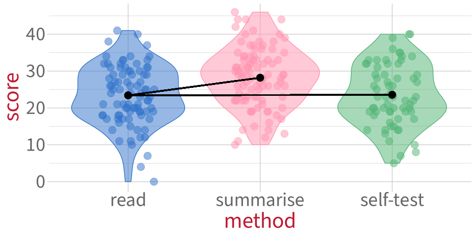
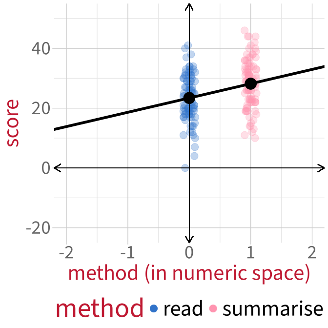
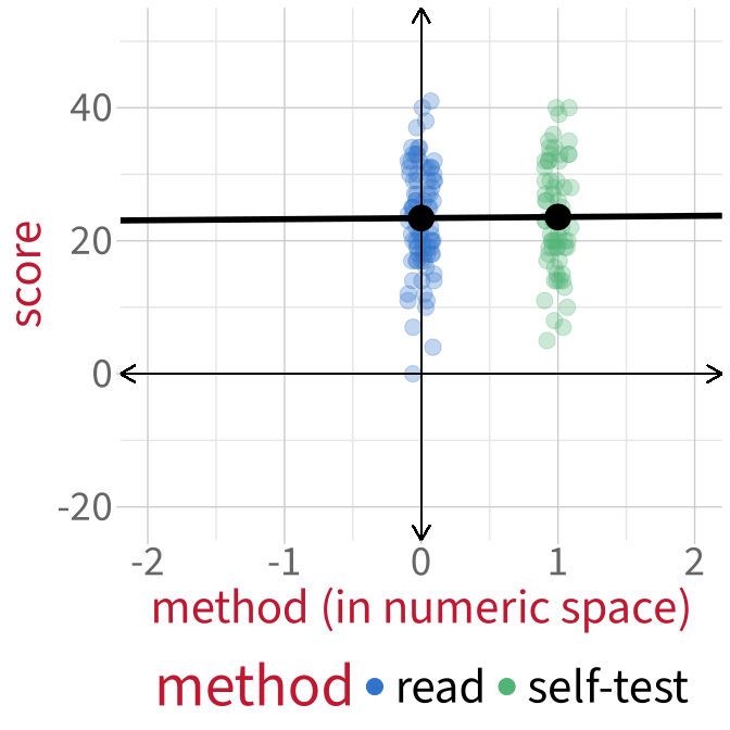
Both dummy variables have the same reference level: read.

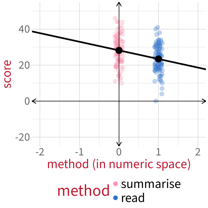
  • The first dummy variable will compare summarise back to read.
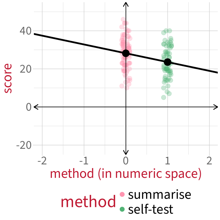
  • The second dummy variable will compare self-test back to read.

Two dummy variables for three levels

First dummy variable: summarise vs. read.

Second dummy variable: self-test vs. read.

How do we know that a model will use these particular dummy variables?


Use contrasts():

contrasts(score_data$method)
          summarise self-test
read              0         0
summarise         1         0
self-test         0         1


How to read this output:

  • Each column contains one dummy variable.
    1. summarise compares summarise (the 1 in that column) to read.
    2. self-test compares self-test (the 1 in that column) to read.
  • We know that the reference level is read because in BOTH dummy variables, read is coded as 0.

Modelling score ~ method

The linear expression:

\[ \text{score} = \beta_0 + (\beta_1 \cdot \text{method}_{\text{summarise}}) + (\beta_2 \cdot \text{method}_{\text{self-test}}) + \epsilon \]

In R:

m3 <- lm(score ~ method, data = score_data)

summary(m3)

Call:
lm(formula = score ~ method, data = score_data)

Residuals:
    Min      1Q  Median      3Q     Max 
-23.414  -5.359  -0.196   5.750  17.804 

Coefficients:
                Estimate Std. Error t value Pr(>|t|)    
(Intercept)       23.414      0.866   27.03  < 2e-16 ***
methodsummarise    4.782      1.193    4.01 0.000081 ***
methodself-test    0.162      1.319    0.12      0.9    
---
Signif. codes:  0 '***' 0.001 '**' 0.01 '*' 0.05 '.' 0.1 ' ' 1

Residual standard error: 8.08 on 247 degrees of freedom
Multiple R-squared:  0.0756,    Adjusted R-squared:  0.0681 
F-statistic: 10.1 on 2 and 247 DF,  p-value: 0.0000605

What does each coefficient mean? (1)

Coefficients:
                 Estimate Std. Error t value Pr(>|t|)    
 (Intercept)       23.414      0.866   27.03  < 2e-16 ***
 methodsummarise    4.782      1.193    4.01 0.000081 ***
 methodself-test    0.162      1.319    0.12      0.9    

(Intercept) aka \(\beta_0\): The mean score for the reference level (read) is 23.41 points.


mean_read
[1] 23.4


  • Null hypothesis: The mean score for the reference level (read) is equal to zero.
  • \(p\)-value: the probability of observing an intercept of 21.41 (or more extreme), assuming that the true intercept is zero.

Can we reject this null hypothesis?


If we care about differences between study methods, is this null hypothesis interesting?

What does each coefficient mean? (2)

Coefficients:
                 Estimate Std. Error t value Pr(>|t|)    
 (Intercept)       23.414      0.866   27.03  < 2e-16 ***
 methodsummarise    4.782      1.193    4.01 0.000081 ***
 methodself-test    0.162      1.319    0.12      0.9    

methodsummarise aka \(\beta_1\): The difference between the estimated average score for summarise and the estimated average score for read is 4.78 points.


mean_summ - mean_read
[1] 4.78


  • Null hypothesis: This difference is equal to zero.
  • \(p\)-value: the probability of a difference of 4.78 (or more extreme), assuming that the true difference is zero.

Can we reject this null hypothesis?


If we care about differences between study methods, is this null hypothesis interesting?

What does each coefficient mean? (3)

Coefficients:
                 Estimate Std. Error t value Pr(>|t|)    
 (Intercept)       23.414      0.866   27.03  < 2e-16 ***
 methodsummarise    4.782      1.193    4.01 0.000081 ***
 methodself-test    0.162      1.319    0.12      0.9    

methodself-test aka \(\beta_2\): The difference between the estimated average score for self-test and the estimated average score for read is 0.16 points.


mean_self - mean_read
[1] 0.162


  • Null hypothesis: This difference is equal to zero.
  • \(p\)-value: the probability of a difference of 0.16 (or more extreme), assuming that the true difference is zero.

Can we reject this null hypothesis?


If we care about differences between study methods, is this null hypothesis interesting?

Changing the reference level

How to change reference level in R?

The original dummy variables:

contrasts(score_data$method)
          summarise self-test
read              0         0
summarise         1         0
self-test         0         1


Reorder factor levels in method, putting our desired reference level first:

score_data <- score_data |>
  mutate(
    method = factor(method, levels = c('summarise', 'read', 'self-test'))
  )


Now check the contrasts. How can we tell that summarise is now the reference level?

contrasts(score_data$method)
          read self-test
summarise    0         0
read         1         0
self-test    0         1

Visualising the new dummy variables

First new dummy variable:

read vs. summarise.

Second new dummy variable:

self-test vs. summarise.

  1. Is the slope of the first dummy variable positive or negative?
  2. Is the slope of the second dummy variable positive or negative?
  3. Will the coefficient estimates be the same or different compared to our previous model?

Old model vs. new model


m4 <- lm(score ~ method, data = score_data)


Reference level = read (old model):

 Coefficients:
                 Estimate Std. Error t value Pr(>|t|)    
 (Intercept)       23.414      0.866   27.03  < 2e-16 ***
 methodsummarise    4.782      1.193    4.01 0.000081 ***
 methodself-test    0.162      1.319    0.12      0.9    


Reference level = summarise (new model):

 Coefficients:
                 Estimate Std. Error t value Pr(>|t|)    
 (Intercept)        28.20       0.82   34.37  < 2e-16 ***
 methodread         -4.78       1.19   -4.01 0.000081 ***
 methodself-test    -4.62       1.29   -3.58  0.00041 ***


Why is methodself-test not significant in the first model, but it IS significant in the second model?

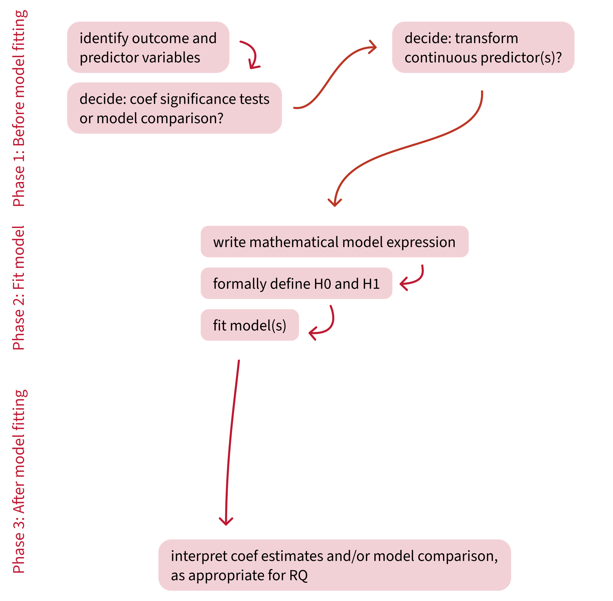
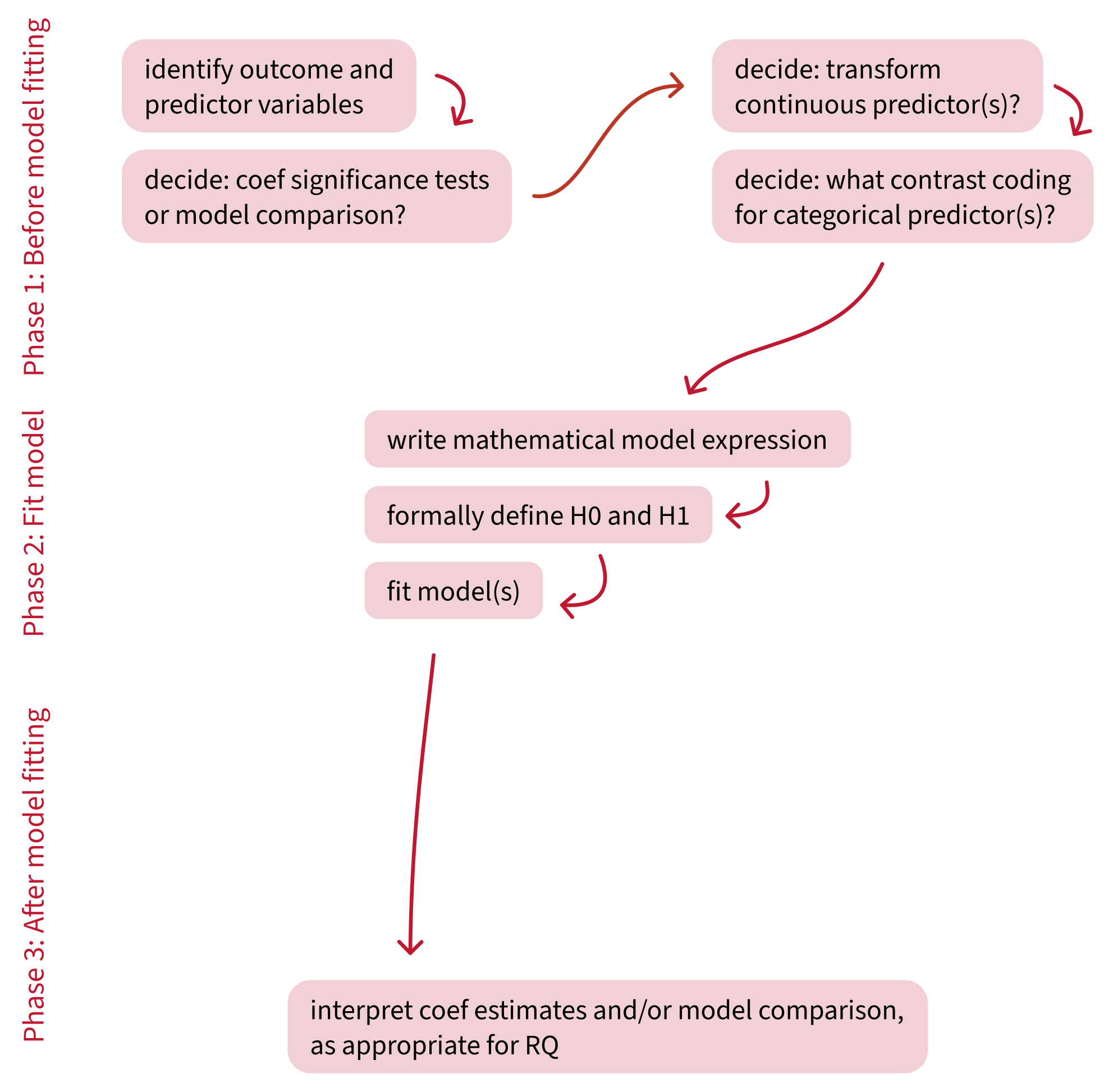
Building an analysis workflow

Building an analysis workflow

Building an analysis workflow

What questions do you have right now?


Back matter

Revisiting this week’s learning objectives

How can we include categorical variables as predictors in a linear model?

  • Represent the variable numerically, for example using treatment coding.
  • In treatment coding, the reference level (also called baseline level) is represented (“coded”) as 0, and the non-reference level is coded as 1.
  • For categorical predictors with >2 levels, multiple “dummy variables” individually compare each non-reference level back to the same reference level.

When we use a categorical predictor, how do we interpret the linear model’s coefficients?

  • Intercept (also written as \(\beta_0\)): The mean outcome for the reference level.
  • Slope (also written as \(\beta_1\), \(\beta_2\), etc., or for short, \(\beta_j\)):
    • the mean outcome for the (current) non-reference level
    • MINUS
    • the mean outcome for the reference level
    • (if multiple regression: while holding other predictors constant)

Revisiting this week’s learning objectives

What hypotheses are tested by the default way that R represents categorical predictors?

  • By default, R uses treatment coding. And by default, the reference level is the level that comes first in the alphabet.
  • The intercept’s H0: The mean outcome for the reference level is equal to zero.
  • The slope’s H0: The difference between the mean outcome for the non-reference level and the mean outcome for the reference level is equal to zero.

What is “contrast coding”?

  • “Contrast coding” is a general term that refers to representing categorical predictors as numbers.
  • One specific example of a contrast coding scheme is treatment coding (which uses 0s and 1s).
  • Another example of a contrast coding scheme is sum coding (which uses –1 and 1). We’ll get to know sum coding next week.

This week


Tasks:


Work on exercises in labs


Complete the weekly quiz

Get support:


Consult the flash cards


Ask questions anonymously on Piazza


We really like seeing you in office hours!

Prediction equations: score ~ study
(two levels)

The linear expression that the model assumes has generated each data point (the reference level is alone:

\[ \text{score} = \beta_0 + (\beta_1 \cdot \text{study}_\text{others}) + \epsilon \]


With simple algebra, we can work out how the \(\beta\) coefficients relate to the estimated score of each group.

Studying alone is represented as \(\text{study}_\text{others}\) = 0.

\[ \begin{align} \text{score}_\text{alone} &= \beta_0 + (\beta_1 \cdot \text{study}_\text{others}) \\ \text{score}_\text{alone} &= \beta_0 + (\beta_1 \cdot 0) \\ \text{score}_\text{alone} &= \beta_0 + 0 \\ \text{score}_\text{alone} &= \beta_0 \\ \end{align} \]

Studying with others is represented as \(\text{study}_\text{others}\) = 1.

\[ \begin{align} \text{score}_\text{others} &= \beta_0 + (\beta_1 \cdot \text{study}_\text{others}) \\ \text{score}_\text{others} &= \beta_0 + (\beta_1 \cdot 1) \\ \text{score}_\text{others} &= \beta_0 + \beta_1 \\ \end{align} \]

Prediction equations: score ~ method
(three levels)

The linear expression that the model assumes has generated each data point (the reference level is read):

\[ \text{score} = \beta_0 + (\beta_1 \cdot \text{method}_\text{self-test}) + (\beta_2 \cdot \text{method}_\text{summarise}) + \epsilon \]


With simple algebra and with the help of the contrasts() function, we can work out how the \(\beta\) coefficients relate to the estimated score of each group.

contrasts(score_data$method)
          self-test summarise
read              0         0
self-test         1         0
summarise         0         1

First: Studying by reading is represented as \(\text{method}_\text{self-test} = 0\) and \(\text{method}_\text{summarise} = 0\).

We get these numbers from the read row of the contrast matrix from contrasts().

\[ \begin{align} \text{score}_\text{read} &= \beta_0 +(\beta_1 \cdot \text{method}_\text{self-test}) + (\beta_2 \cdot \text{method}_\text{summarise}) \\ \text{score}_\text{read} &= \beta_0 + (\beta_1 \cdot 0) + (\beta_2 \cdot 0) \\ \text{score}_\text{read} &= \beta_0 + 0 + 0 \\ \text{score}_\text{read} &= \beta_0 \\ \end{align} \]

Prediction equations: score ~ method
(three levels)


contrasts(score_data$method)
          self-test summarise
read              0         0
self-test         1         0
summarise         0         1

Second: Studying by self-testing is represented as \(\text{method}_\text{self-test} = 1\) and \(\text{method}_\text{summarise} = 0\).

We get these numbers from the self-test row of the contrast matrix from contrasts().

\[ \begin{align} \text{score}_\text{self} &= \beta_0 +(\beta_1 \cdot \text{method}_\text{self-test}) + (\beta_2 \cdot \text{method}_\text{summarise}) \\ \text{score}_\text{self} &= \beta_0 +(\beta_1 \cdot 1) + (\beta_2 \cdot 0) \\ \text{score}_\text{self} &= \beta_0 + \beta_1 + 0 \\ \text{score}_\text{self} &= \beta_0 + \beta_1\\ \end{align} \]

Prediction equations: score ~ method
(three levels)


contrasts(score_data$method)
          self-test summarise
read              0         0
self-test         1         0
summarise         0         1

Third: Studying by summarising is represented as \(\text{method}_\text{self-test} = 0\) and \(\text{method}_\text{summarise} = 1\).

We get these numbers from the summarise row of the contrast matrix from contrasts().

\[ \begin{align} \text{score}_\text{summ} &= \beta_0 +(\beta_1 \cdot \text{method}_\text{self-test}) + (\beta_2 \cdot \text{method}_\text{summarise}) \\ \text{score}_\text{summ} &= \beta_0 +(\beta_1 \cdot 0) + (\beta_2 \cdot 1) \\ \text{score}_\text{summ} &= \beta_0 + 0 + \beta_2 \\ \text{score}_\text{summ} &= \beta_0 + \beta_2 \\ \end{align} \]

Why bother with a reference level?

Why can’t we just compare each group individually to the overall mean?

Such a model might look something like this:

\[ \text{score} = \beta_0 + (\beta_1 \cdot \text{read}) + (\beta_2 \cdot \text{selftest}) + (\beta_3 \cdot \text{summarise}) + \epsilon \]

Each score is given by an intercept plus the difference between that intercept and each group’s scores. The mean \(\mu\) of each group would be:

\[ \begin{align} \mu_\text{read} &= \beta_0 + (\beta_1 \cdot \text{read})\\ \mu_\text{selftest} &= \beta_0 + (\beta_2 \cdot \text{selftest})\\ \mu_\text{summarise} &= \beta_0 + (\beta_3 \cdot \text{summarise})\\ \end{align} \]

For technical reasons, we cannot model this data this way.

We are trying to estimate three group means: \(\mu_\text{read}\), \(\mu_\text{selftest}\), \(\mu_\text{summarise}\). And for mathematical reasons, that means we can only have three parameters in our model. But the model above has four: \(\beta_0\), \(\beta_1\), \(\beta_2\), \(\beta_3\).

In technical terms, we say the model above is overparameterised.


Treatment coding with a reference level is one way to achieve three parameters for three group means: one intercept for the reference level and two differences between groups for the other two levels.