Testing Predictors and Evaluating Linear Models

Data Analysis for Psychology in R 2

Dr. Patrick Sturt (Patrick.Sturt@ed.ac.uk)

Department of Psychology
University of Edinburgh
2026–2027

Course overview

Introduction to linear models (with Dr. Patrick Sturt)	Introduction to linear regression
	Interpreting linear models
	Testing predictors and evaluating linear models
	F-tests and model comparison
	Practice analysis: Linear models
Extending linear models (with Dr. Elizabeth Pankratz)	Categorical predictors and treatment coding
	Sum coding
	Assumptions and diagnostics
	Bootstrapping and confidence intervals
	Practice analysis: Categorical predictors (led by Patrick)

Interactions (with Dr. Elizabeth Pankratz)	Mean-centering and numeric/categorical interactions
	Numeric/numeric interactions
	Categorical/categorical interactions
	Testing simple effects and correcting for multiple comparisons
	Practice analysis: Interactions (led by Patrick)
Logistic regression (with Dr. Elizabeth Pankratz)	Probabilities and log-odds
	Modelling binary outcomes with logistic regression
	Interactions, assumptions, diagnostics, comparisons
	Practice analysis: Logistic regression (led by Patrick)
	Report feedback, exam prep, full-course Q&A

This Week’s Learning Objectives

1. Understand how to interpret significance tests for \(\beta\) coefficients

2. Understand how to calculate and interpret \(R^2\) and adjusted- \(R^2\) as a measure of model quality

3. Be able to locate information on the significance of individual predictors and overall model fit in R lm model output

Part 1: Recap & Overview

Recap

• Last week we expanded the general linear model equation to include multiple predictors:

\[ y_i = \beta_0 + (\beta_1 \cdot x_{1i}) + (\beta_2 \cdot x_{2i}) + (\beta_j \cdot x_{ji}) + \epsilon_i \]

• And we ran an example concerning test scores:

\[ \text{Score}_i = \beta_0 + (\beta_1 \cdot \text{Hours}_{i}) + (\beta_2 \cdot \text{Motivation}_{i}) + \epsilon_i \]

• And we looked at how to run this model in R:

lm(score ~ hours + motivation, data = test_study2)

Evaluating our Model

So far we have estimated values for the key parameters of our model ( \(\beta\)s )

• Now we have to think about how we evaluate the model

• Evaluating a model will consist of:

  1. Evaluating the individual coefficients

  2. Evaluating the overall model quality

  3. Evaluating the model assumptions

Important: Before accepting a set of results, all three of these aspects of evaluation must be considered

• We will talk about evaluating individual coefficients and model quality today
• Model assumptions covered later in the course (Semester 1, Week 8)

Significance of Individual Effects

• A general way to ask this question would be to state:

Is our model informative about the association between X and Y?

• In the context of our example from last lecture, we could ask,

Is study time a useful predictor of test score?

• This is kind of vague, what does it mean to be a “useful predictor”?

• We need to turn this into a testable statistical hypothesis

Evaluating Individual Predictors

Steps in hypothesis testing:

• Research question

• Statistical hypothesis

• Define the null hypothesis

• Calculate an estimate of effect of interest

• Calculate an appropriate test statistic

• Evaluate the test statistic against the null

Research Questions and Hypotheses

Research questions are statements of what we intend to study

A good question defines:

• constructs under study
• the association being tested
• a direction of association
• target populations etc.

For example:

Does increased study time improve test scores in school-age children?

Research Questions and Hypotheses

Statistical hypotheses are testable mathematical statements

• In typical testing in Psychology, we define a null hypothesis (\(H_0\)) and an alternative hypothesis (\(H_1\)).

  • \(H_0\) is precise: it specifically states that the effect of interest is equal to zero.
  • \(H_1\) is not specific: it simply says that the effect of interest is not equal to zero (but it makes no claims about what the effect of interest might really be equal to).

Statistical Significance: Review from DAPR1

• Remember, we can only ever test the null hypothesis

• We select a significance level, \(\alpha\) (typically .05)

• Then we calculate the \(p\)-value associated with our test statistic

  • A \(p\)-value is the probability of observing our test statistic or a value even more extreme than our test statistic, assuming that \(H_0\) is true (that is, assuming that the true effect really is zero)

• If the associated \(p\) is smaller than \(\alpha\), then we reject the null

• If it is larger, then we fail to reject the null

Part 2: Steps in Significance Testing

Defining the Null

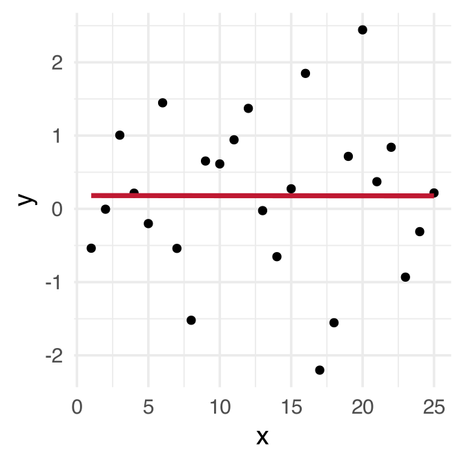
In this example data, there’s no pattern in how values of \(x\) are associated with values of \(y\).

We can’t make any guesses about \(y\) based on the value of \(x\).

In this scenario, the slope \(\beta_1\) of the line associating \(x\) and \(y\) is 0.

Why is the slope 0?

• \(\beta\) gives the predicted change in \(y\) for a unit change in \(x\)
• If \(x\) and \(y\) are unrelated, then a change in \(x\) will not result in any change to the predicted value of \(y\)
• So for a unit change in \(x\), there is no change (zero change) in \(y\)

Our null hypothesis is that there is no association between \(x\) and \(y\). Formally:

\[H_0: \beta_1 = 0\] \[H_1: \beta_1 \neq 0\]

Significance tests for \(\beta\) coefficients

• The test statistic associated with \(\beta\) coefficients is a \(t\)-statistic:

\[t = \frac{\beta}{SE(\beta)} = \frac{\text{estimated coefficient}}{\text{standard error estimated for that coefficient}}\]

• Recall from DAPR1 that the standard error describes the spread of the sampling distribution
  • The standard error \((SE)\) measures how variable the sample is
  • A smaller SE suggests a more precise estimate (= good)
  • If you like maths, check the appendix of these slides for details about how to compute SE by hand

Let’s work out a \(t\)-value

summary(m1)

Call:
lm(formula = score ~ hours + motivation, data = test_study2)

Residuals:
     Min       1Q   Median       3Q      Max 
-12.9548  -2.8042  -0.2847   2.9344  13.8240 

Coefficients:
            Estimate Std. Error t value Pr(>|t|)    
(Intercept)  6.86679    0.65473  10.488   <2e-16 ***
hours        1.37570    0.07989  17.220   <2e-16 ***
motivation   0.91634    0.38376   2.388   0.0182 *  
---
Signif. codes:  0 '***' 0.001 '**' 0.01 '*' 0.05 '.' 0.1 ' ' 1

Residual standard error: 4.386 on 147 degrees of freedom
Multiple R-squared:  0.6696,    Adjusted R-squared:  0.6651 
F-statistic: 148.9 on 2 and 147 DF,  p-value: < 2.2e-16

For motivation, which we’ll represent as \(\beta_2\):

\[ t = \frac{\beta_2}{SE(\beta_2)} = \frac{0.9163}{0.3838} = 2.388 \]

Compare \(t\) to a Null Distribution

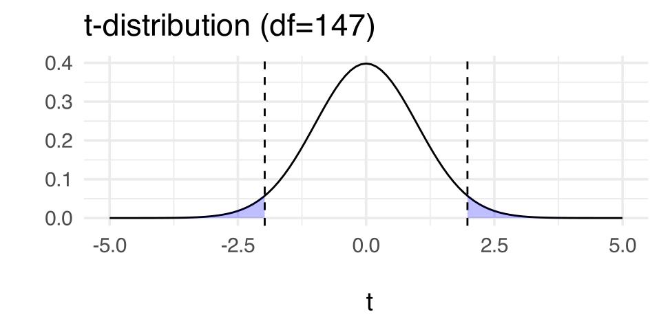
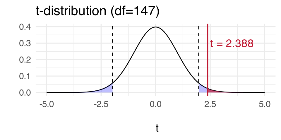
• We have an observed \(t\)-statistic, 2.388. Now we want to find out how likely it is to observe a \(t\)-value this extreme or more extreme, assuming that \(H_0\) is true.

• We know the distribution that \(t\)-values follow when \(H_0\) is true: a \(t\)-distribution.

• \(t\)-distributions can vary, depending on their degrees of freedom (df):

• For \(\beta\), the null distribution is a \(t\)-distribution with \(n-k-1\) degrees of freedom
  • \(n\) = sample size
  • \(k\) = number of predictors (that is, the number of \(\beta\) coefficients that are not the intercept \(beta_0\))
    • The additional –1 represents the intercept

\(n-k-1\) degrees of freedom

• \(n\) = sample size = 150
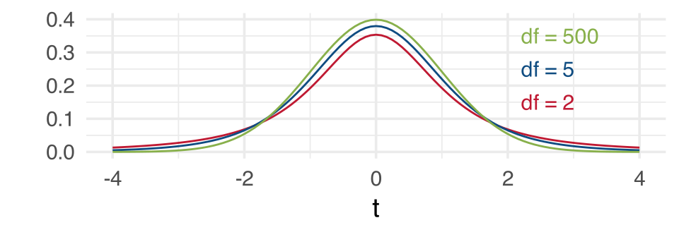
• \(k\) = number of predictors = 2 (hours and motivation)

So: \(150 - 2 - 1 = 147\) degrees of freedom.

Use null distribution to find critical values

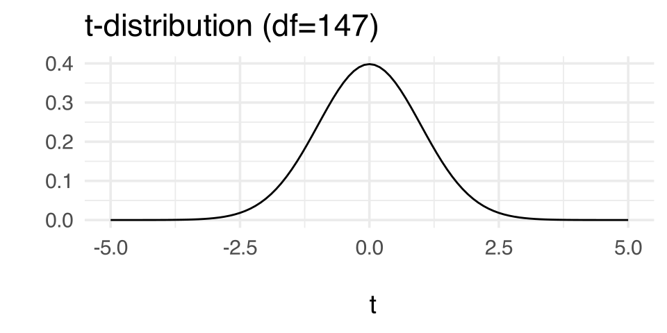
• As with all tests we need to set our \(\alpha\): our probability of incorrectly rejecting the null hypothesis, even when it’s true

  • Let’s set \(\alpha\) = 0.05 (two tailed)
  • This is a 5% risk of incorrectly rejecting the null

• We’ll use this \(\alpha\) value, together with the null distribution from the last slide, to find the critical values that we’ll compare our observed \(t\)-value to

Critical values

• Critical values \((t^*)\) establish a boundary for significance
• The probability that a \(t\)-value will fall within these extreme regions of the distribution given \(H_0\) is true is equal to \(\alpha\)
• Because we are performing a two-tailed test, \(\alpha\) is split between each tail, and the critical values are the edges of that shaded region (the dashed lines).

c(
  lower = round(qt(0.025, 147), 3),
  upper = round(qt(0.975, 147), 3)
)

 lower  upper 
-1.976  1.976 

How our \(t\)-value of 2.388 compares

The shaded red area, times 2 because it’s a two-tailed test, gives us a \(p\)-value of .018.

\(p = .018\) is less than \(\alpha = 0.05\), so we can reject the null hypothesis that the association between motivation and score is equal to zero.

Part 3: Measure Model Quality using the Coefficient of Determination ( \(R^2\) )

Quality of the Overall Model

• When we measure an outcome variable \(y\), there will be variability in that outcome.

  • Some variability arises (we hope) because an independent variable \(x\) impacts \(y\).
    • This is variability our model can explain.
  • Other variability arises because there is just random variability in the world that we can’t possibly account for.
    • This is variability our model cannot explain.

• We quantify how good our model is based on what proportion of the variability in our data it can explain.

What proportion of variability the model can explain

To work out this proportion, we need to quantify three different kinds of variability:

Type of variability in \(y\)	How we quantify it
Variability explained by model	\(SS_{Model}\) “Model sum of squares”
Variability not explained by model	\(SS_{Residual}\) “Residual sum of squares”
Total variability	\(SS_{Model} + SS_{Residual} = SS_{Total}\) “Total sum of squares”

The proportion of variability that the model explains is then computed as

\[\frac{SS_{Model}}{SS_{Total}} \quad \text{or} \quad 1 - \frac{SS_{Residual}}{SS_{Total}}\]

We call this proportion the coefficient of determination and represent it as \(R^2\).

Interpreting the Coefficient of Determination

\[ \begin{align} R^2 &= \frac{SS_{Model}}{SS_{Total}}\\[1em] &= 1 - \frac{SS_{Residual}}{SS_{Total}} \\ \end{align} \]

• Quantifies the amount of variability in the outcome accounted for by the predictors
• The more variance accounted for, the better the model fit
• Represents the extent to which the prediction of \(y\) is improved when predictions are based on the linear relation between \(x\) and \(y\), compared to not considering \(x\)

Let’s see how to calculate each of these three sums of squares.

Total Sum of Squares: Distance from mean

\[SS_{Total} = \sum_{i=1}^{n}(y_i - \bar{y})^2\]

In words: For every observation, find the difference between the observed value and the mean of all observed \(y\) values, square that difference, and add up all the squares.

Residual Sum of Squares: Distance from model

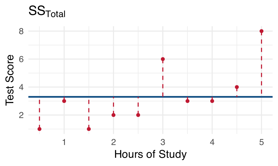
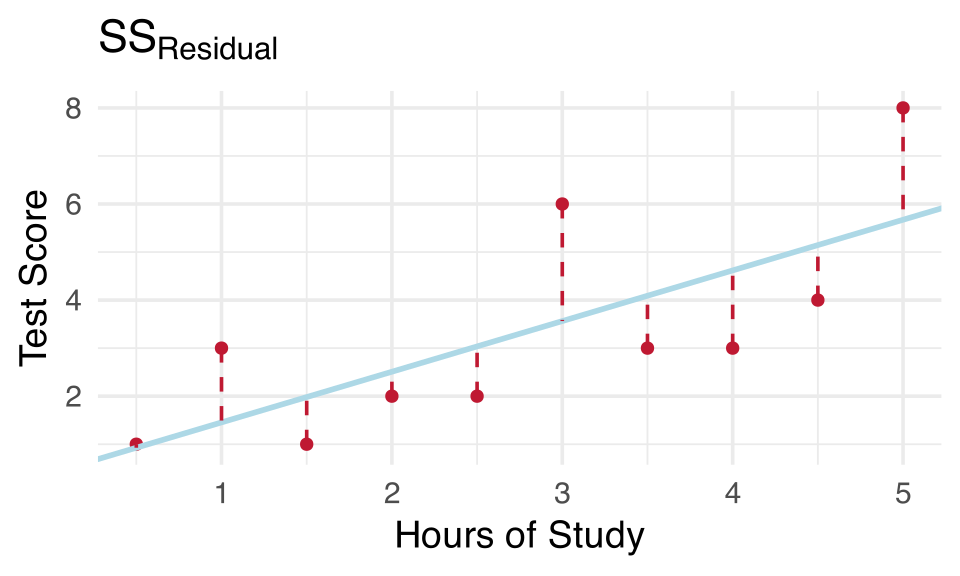
\[SS_{Residual} = \sum_{i=1}^{n}(y_i - \hat{y}_i)^2\]

In words: For every observation, find the difference between that observation and the value predicted by the model, square that difference, and add up all the squares.

Model Sum of Squares: Distance between model and mean

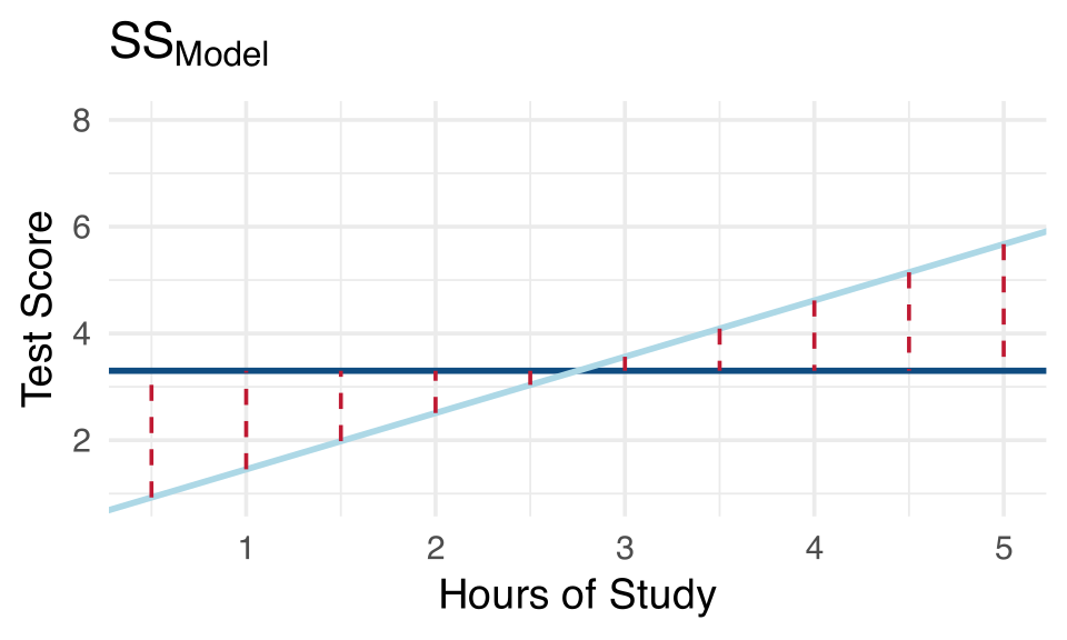
\[SS_{Model} = \sum_{i=1}^{n}(\hat{y}_i - \bar{y})^2\]

In words: For every observation, find the difference between the predicted value for that observation and the mean of all observed \(y\) values, square that difference, and add them all up.

Our model’s \(R^2\)

• In the current example, these values are:

  • \(SS_\text{total}\) = 8556.06
  • \(SS_\text{residual}\) = 2826.83
  • \(SS_\text{model}\) = 5729.23

\[ R^2 = \frac{SS_{Model}}{SS_{Total}} \]

\[ \begin{align} R^2 &= \frac{5729.23}{8556.06} \\[.5em] &= 0.6695 \\ \end{align} \]

\(R^2\) = 0.6695 means that 66.95% of the variation in test scores is accounted for by hours of revision and student motivation

This \(R^2\) = lm()’s Multiple R-squared!
(with some rounding error)

summary(m1)

Call:
lm(formula = score ~ hours + motivation, data = test_study2)

Residuals:
     Min       1Q   Median       3Q      Max 
-12.9548  -2.8042  -0.2847   2.9344  13.8240 

Coefficients:
            Estimate Std. Error t value Pr(>|t|)    
(Intercept)  6.86679    0.65473  10.488   <2e-16 ***
hours        1.37570    0.07989  17.220   <2e-16 ***
motivation   0.91634    0.38376   2.388   0.0182 *  
---
Signif. codes:  0 '***' 0.001 '**' 0.01 '*' 0.05 '.' 0.1 ' ' 1

Residual standard error: 4.386 on 147 degrees of freedom
Multiple R-squared:  0.6696,    Adjusted R-squared:  0.6651 
F-statistic: 148.9 on 2 and 147 DF,  p-value: < 2.2e-16

What’s Adjusted \(R^2\)?

• When there are two or more predictors, \(R^2\) tends to be an inflated estimate of the corresponding population value

  • Due to random sampling fluctuation, even when \(R^2 = 0\) in the population, it’s value in the sample may \(\neq 0\)

  • In smaller samples, the fluctuations from zero will be larger on average

  • With more predictors, there are more opportunities to add to the positive fluctuation

• We therefore compute an adjusted \(R^2\)

\[ \hat R^2 = 1 - (1 - R^2)\frac{n-1}{n-k-1} \]

• Adjusted \(R^2\) adjusts for both sample size \(n\) and number of predictors \(k\)

Our Multiple R-squared vs. Adjusted R-squared

 Residual standard error: 4.386 on 147 degrees of freedom
 Multiple R-squared:  0.6696,   Adjusted R-squared:  0.6651 
 F-statistic: 148.9 on 2 and 147 DF,  p-value: < 2.2e-16
 

• Based on adjusted R-squared, hours studying and student motivation explain 66.5% of the variance in test scores

• As the sample size is large and the number of predictors small, unadjusted (0.67) and adjusted R-squared (0.665) are similar

• If there were even more predictors, then adjusted R-squared would be a much more accurate representation of proportion variance explained

Summary

• We have an inferential test, based on a \(t\)-distribution, for the significance of \(\beta\)

• We are more likely to find a statistically significant effect when residuals are small and we have a large sample

• We can assess the degree to which our model explains variance in the outcome based on \(R^2\)

• When we have multiple predictors, we should use the adjusted \(R^2\) to get a more conservative estimate

Back matter

This week

Tasks:

Work on exercises in labs

Complete the weekly quiz

Get support:

Consult the flash cards

Ask questions anonymously on Piazza

We really like seeing you in office hours!

Appendix

Standard error: The maths

• The formula for the standard error of the slope is:

\[ SE(\beta_j) = \sqrt{\frac{ SS_{Residual}/(n-k-1)}{\sum(x_{ij} - \bar{x_{j}})^2(1-R_{xj}^2)}} \]

• Where:
  • \(SS_{Residual}\) is the residual sum of squares
  • \(n\) is the sample size
  • \(k\) is the number of predictors
  • \(x_{ij}\) is the observed value of a predictor ( \(j\) ) for an individual ( \(i\) )
  • \(\bar{x_{j}}\) is the mean of a predictor
  • \(R_{xj}^2\) derives from the multiple correlation coefficient of the predictors
• \(R_{xj}^2\) captures to degree to which all of our predictors are related to each other
  • For simple linear models, \(R_{xj}^2\) = 0 as there is only 1 predictor

SE( \(\beta_j\) )

\[ SE(\beta_j) = \sqrt{\frac{ SS_{Residual}/(n-k-1)}{\sum(x_{ij} - \bar{x_{j}})^2(1-R_{xj}^2)}} \]

• We want our \(SE\) to be smaller - this means our estimate is precise

• Examining the above formula we can see that:

  • \(SE\) is smaller when residual variance ( \(SS_{residual}\) ) is smaller
  • \(SE\) is smaller when sample size ( \(n\) ) is larger
  • \(SE\) is larger when the number of predictors ( \(k\) ) is larger
  • \(SE\) is larger when a predictor is strongly correlated with other predictors ( \(R_{xj}^2\) )