lm(DV ~ IV, data = datasetName)Interpreting Linear Models
Data Analysis for Psychology in R 2
Dr. Patrick Sturt (Patrick.Sturt@ed.ac.uk)
Department of Psychology
University of Edinburgh
2026–2027
Course overview
|
Introduction to linear models (with Dr. Patrick Sturt) |
Introduction to linear regression |
| Interpreting linear models | |
| Testing predictors and evaluating linear models | |
| F-tests and model comparison | |
| Practice analysis: Linear models | |
|
Extending linear models (with Dr. Elizabeth Pankratz) |
Categorical predictors and treatment coding |
| Sum coding | |
| Assumptions and diagnostics | |
| Bootstrapping and confidence intervals | |
| Practice analysis: Categorical predictors (led by Patrick) |
|
Interactions (with Dr. Elizabeth Pankratz) |
Mean-centering and numeric/categorical interactions |
| Numeric/numeric interactions | |
| Categorical/categorical interactions | |
| Testing simple effects and correcting for multiple comparisons | |
| Practice analysis: Interactions (led by Patrick) | |
|
Logistic regression (with Dr. Elizabeth Pankratz) |
Probabilities and log-odds |
| Modelling binary outcomes with logistic regression | |
| Interactions, assumptions, diagnostics, comparisons | |
| Practice analysis: Logistic regression (led by Patrick) | |
| Report feedback, exam prep, full-course Q&A |
This Week’s Learning Objectives
Be able to interpret the coefficients from a simple linear model
Understand how and why we standardise coefficients and how this impacts interpretation
Understand how these interpretations change when we add more predictors
Part 1: Recap & Coefficient Interpretation
Linear Model
- Last week we introduced the linear model:
\[y_i = \beta_0 + \beta_1 x_{i} + \epsilon_i\]
- Where:
- \(y_i\) is our measured outcome variable
- \(x_i\) is our measured predictor variable
- \(\beta_0\) is the model intercept
- \(\beta_1\) is the model slope
- \(\epsilon_i\) is the residual error (difference between the model predicted and the observed value of \(y\))
- We spoke about calculating by hand, and also the key concept of residuals
lm in R
- You also saw the basic structure of the
lm()function:
- And we ran our first model:
Call:
lm(formula = score ~ hours, data = test)

Coefficients:
(Intercept)        hours
0.400 1.055 - This week, we are going to focus on the interpretation of our model, and how we extend it to include more predictors
lm in R
Call:
lm(formula = score ~ hours, data = test)

Residuals:
    Min      1Q  Median      3Q     Max
-1.6182 -1.0773 -0.7454  1.1773  2.4364

Coefficients:
            Estimate Std. Error t value Pr(>|t|)
(Intercept)   0.4000     1.1111   0.360   0.7282
hours         1.0545     0.3581   2.945   0.0186 *
---
Signif. codes:  0 '***' 0.001 '**' 0.01 '*' 0.05 '.' 0.1 ' ' 1

Residual standard error: 1.626 on 8 degrees of freedom
Multiple R-squared:  0.5201,    Adjusted R-squared:  0.4601
F-statistic:  8.67 on 1 and 8 DF,  p-value: 0.01858
Interpretation
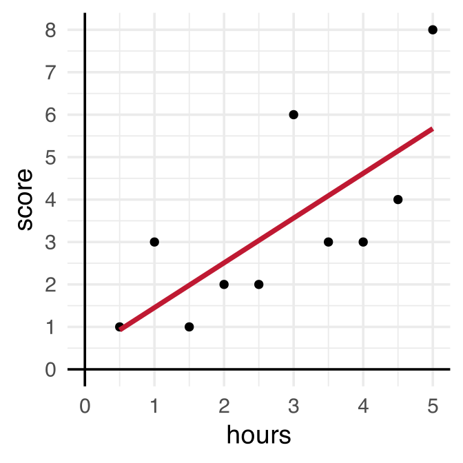
Coefficients:
             Estimate Std. Error t value Pr(>|t|)
 (Intercept)   0.4000     1.1111   0.360   0.7282
hours 1.0545 0.3581 2.945 0.0186 *(Intercept)= the expected outcome value Y when the predictor X is 0- X = 0 represents zero hours of studying (
hours= 0) - As the intercept is 0.400, we conclude that a student who does not study would be expected to score 0.40 on the test
- X = 0 represents zero hours of studying (
hours= slope = how much the outcome Y increases, on average, when the predictor X increases by one unit- Unit of Y = 1 point on the test
- Unit of X = 1 hour of study
- As the slope for
hoursis 1.055, we conclude that for every hour of study, test score increases on average by 1.055 points
- Unit of Y = 1 point on the test
Note of Caution on Interpreting Intercepts
In our example, 0 has a meaning
- It is a student who has studied for 0 hours
But it is not always the case that 0 is meaningful
Suppose our predictor variable was not hours of study, but age
If the predictor was age, how would we interpret an intercept of 0.4? What does age = 0 mean?
This is a general lesson about interpreting statistical tests:
- The interpretation is always in the context of the constructs and how we have measured them
Practice with Scales of Measurement (1)
Imagine a model looking at the association between an employee’s salary \(y\) and their duration of employment \(x\):
\[y_i = \beta_0 + \beta_1 x_{i} + \epsilon_i\]
- \(x\) = unit is 1 year
- \(y\) = unit is £1000
- \(\beta_1\) = 0.4
- In this context, what does each coefficient mean?
- \(\beta_0\)?
- \(\beta_1\)?
- \(\beta_0\)?
For reference/hint:
\(\beta_0\) = intercept = expected value of Y when X is 0
\(\beta_1\) = slope = how many units Y increases, on average, for a unit increase in X
Practice with Scales of Measurement (2)
Imagine a model looking at the association between the length of cats’ tails \(y\) and their weight \(x\):
\[y_i = \beta_0 + \beta_1 x_{i} + \epsilon_i\]
- \(x\) = unit is 1kg
- \(y\) = unit is 1cm
- \(\beta_1\) = -3.2
- In this context, what does each coefficient mean?
- \(\beta_0\)?
- \(\beta_1\)?
- \(\beta_0\)?
For reference/hint:
\(\beta_0\) = intercept = expected value of Y when X is 0
\(\beta_1\) = slope = how many units Y increases, on average, for a unit increase in X
Practice with Scales of Measurement (3)
Imagine a model looking at the association between healthy eating habits \(y\) and conscientiousness \(x\):
\[y_i = \beta_0 + \beta_1 x_{i} + \epsilon_i\]
- \(x\) = unit is 1 increment on a Likert scale ranging from 1 to 5 measuring conscientiousness
- \(y\) = unit is 1 increment on a healthy eating scale
- \(\beta_1\) = 0.25
- In this context, what does each coefficient mean?
- \(\beta_0\)?
- \(\beta_1\)?
- \(\beta_0\)?
For reference/hint:
\(\beta_0\) = intercept = expected value of Y when X is 0
\(\beta_1\) = slope = how many units Y increases, on average, for a unit increase in X
Part 2: Standardisation
Unstandardised vs Standardised Coefficients
- So far we have interpreted the coefficients using the units in which they were originally measured
- We interpreted the slope as the change in \(y\) units for a unit change in \(x\) , where the unit is determined by how we have measured our variables
- We call these coefficients unstandardised
- We interpreted the slope as the change in \(y\) units for a unit change in \(x\) , where the unit is determined by how we have measured our variables
- However, sometimes these units are not helpful for interpretation
- We can then perform standardisation to aid interpretation
Standardised Units
Why might standard units be useful?
- If the scales of our variables are arbitrary
- Example: A sum score of questionnaire items answered on a Likert scale.
- A unit here would equal moving from e.g. a 2 to 3 on one item
- This is not especially meaningful (and actually has A LOT of associated assumptions)
- If we want to compare the effects of variables on different scales
- If we want to say something like “the effect of \(x_1\) is stronger than the effect of \(x_2\)”, we need a common scale
Option 1: Standardising the coefficients after fitting the model
- After calculating a \(\beta_1\), it can be standardised by:
\[{\beta_1^*} = \beta_1 \frac{s_x}{s_y} = \text{unstandardised coef} \times \frac{\text{SD of predictor}~x}{\text{SD of outcome}~y}\]
Defining each variable:
- \({\beta_1^*}\) = standardised beta coefficient
- \(\beta_1\) = unstandardised beta coefficient
- \(s_x\) = standard deviation of \(x\)
- \(s_y\) = standard deviation of \(y\)
Implementing in R
- Step 1: Obtain coefficients from the model
            Estimate Std. Error   t value  Pr(>|t|)
(Intercept) 0.400000  1.1111010 0.3600033 0.7281636
hours 1.054545 0.3581403 2.9445039 0.0185812Option 2: Standardising the variables before fitting the model
Another option is to transform continuous predictor and outcome variables to \(z\)-scores (mean=0, SD=1) prior to fitting the model
If both \(x\) and \(y\) are standardised, our model coefficients (betas) are standardised too
\(z\)-score for \(x\):
\[z_{x_i} = \frac{x_i - \bar{x}}{s_x} = \frac{\text{observed value of}~x~\text{minus mean of}~x}{\text{SD of}~x}\]
- and the \(z\)-score for \(y\):
\[z_{y_i} = \frac{y_i - \bar{y}}{s_y} = \frac{\text{observed value of}~y~\text{minus mean of}~y}{\text{SD of}~y}\]
- That is, we divide each observation’s deviation from the mean by the standard deviation
Implementing in R
- Step 1: Convert predictor and outcome variables to z-scores by subtracting the mean and dividing the difference by the SD
Interpreting Standardised Coefficients
Unstandardised
Call:
lm(formula = score ~ hours, data = test)

Residuals:
    Min      1Q  Median      3Q     Max
-1.6182 -1.0773 -0.7454  1.1773  2.4364

Coefficients:
            Estimate Std. Error t value Pr(>|t|)
(Intercept)   0.4000     1.1111   0.360   0.7282
hours         1.0545     0.3581   2.945   0.0186 *
---
Signif. codes:  0 '***' 0.001 '**' 0.01 '*' 0.05 '.' 0.1 ' ' 1

Residual standard error: 1.626 on 8 degrees of freedom
Multiple R-squared:  0.5201,    Adjusted R-squared:  0.4601
F-statistic:  8.67 on 1 and 8 DF,  p-value: 0.01858
Standardised
Call:
lm(formula = score_z ~ hours_z, data = test)

Residuals:
    Min      1Q  Median      3Q     Max
-0.7310 -0.4867 -0.3368  0.5318  1.1006

Coefficients:
             Estimate Std. Error t value Pr(>|t|)
(Intercept) 1.172e-17  2.324e-01   0.000   1.0000
hours_z     7.212e-01  2.449e-01   2.945   0.0186 *
---
Signif. codes:  0 '***' 0.001 '**' 0.01 '*' 0.05 '.' 0.1 ' ' 1

Residual standard error: 0.7348 on 8 degrees of freedom
Multiple R-squared:  0.5201,    Adjusted R-squared:  0.4601
F-statistic:  8.67 on 1 and 8 DF,  p-value: 0.01858
Interpreting Standardised Coefficients
(Intercept):
- The intercept is always zero when all variables are standardised (because their means all become zero). The math, if you’re interested:
\[ \begin{align} \beta_0 &= \bar{y}-\beta_1\bar{x} \\ &= 0 - \beta_1 0 \\ &= 0 \end{align} \]
Slope:
The interpretation of the slope coefficient(s) becomes the increase in \(y\) in standard deviation units for every standard deviation increase in \(x\)
So, in our example:
For every standard deviation increase in hours of study, test score increases by 0.72 standard deviations
Which Should we use?
- Unstandardised regression coefficients are often more useful when the variables are on meaningful scales
- E.g. X additional hours of exercise per week adds Y years of healthy life
- Sometimes it’s useful to obtain standardised regression coefficients
- When the scales of variables are arbitrary
- When there is a desire to compare the effects of variables measured on different scales
- Cautions
- Just because you can put regression coefficients on a common metric doesn’t mean they can be meaningfully compared
- The SD is a poor measure of spread for skewed distributions, therefore, be cautious of their use with skewed variables
Relationship to Correlation ( \(r\) )
- If a linear model has a single, continuous predictor, then the standardised slope ( \(\beta_1^*\) ) is actually exactly the same as the correlation coefficient ( \(r\) ) between the predictor and the outcome!
- For example:
Relationship to Correlation ( \(r\) )
- They are equivalent:
- \(r\) is a standardised measure of linear association
- \(\beta_1^*\) is a standardised measure of the linear slope
- Similar idea for linear models with multiple predictors
- Slopes are now equivalent to the part correlation coefficient
Part 3: Multiple Regression
Multiple Predictors
The aim of a linear model is to explain variance in an outcome
In simple linear models, we have a single predictor, but the model can accommodate (in principle) any number of predictors
If we have multiple predictors for an outcome, those predictors may be correlated with each other
A linear model with multiple predictors finds the optimal prediction of the outcome from several predictors, taking into account their redundancy with one another
Uses of Multiple Regression
For prediction: multiple predictors may lead to improved prediction
For theory testing: often our theories suggest that multiple variables together contribute to variation in an outcome
For covariate control: we might want to assess the effect of a specific predictor, controlling for the influence of others
- E.g., effects of personality on health after removing the effects of age and gender
Extending the Regression Model
- Our model for a single predictor:
\[y_i = \beta_0 + (\beta_1 \cdot x_{1i}) + \epsilon_i\]
- is extended to include additional \(x\)’s:
\[y_i = \beta_0 + (\beta_1 \cdot x_{1i}) + (\beta_2 \cdot x_{2i}) + (\beta_3 \cdot x_{3i}) + \epsilon_i\]
- For each \(x\), we have an additional \(\beta\)
- \(\beta_1\) is the slope coefficient for the first predictor
- \(\beta_2\) for the second etc.
Interpreting Coefficients in Multiple Regression
\[y_i = \beta_0 + (\beta_1 \cdot x_{1i}) + (\beta_2 \cdot x_{2i}) + ~~ ... ~ + (\beta_j \cdot x_{ji}) + \epsilon_i\]
Given that we have additional variables, our interpretation of the regression coefficients changes a little
\(\beta_0\) = the predicted value for \(y\) when all \(x\) are 0
Each \(\beta_j\) is now a partial regression coefficient
- It captures the change in \(y\) for a one unit change in \(x\) when all other x’s are held constant
What does “holding constant” mean?
What Does “Holding Constant” Mean?
Refers to finding the effect of the predictor when the values of the other predictors are fixed
With multiple predictors
lmisolates the effects and estimates the unique contributions of predictors
You might also hear the same idea referred to with other language, e.g.:
- “controlling for other predictors” \(\leftarrow\) we’ll use this one mostly!
- “adjusting for other predictors”
- “partialling out other predictors”
- “residualising for other predictors”
Visualising Models
A linear model with one continuous predictor: two-dimensional line.
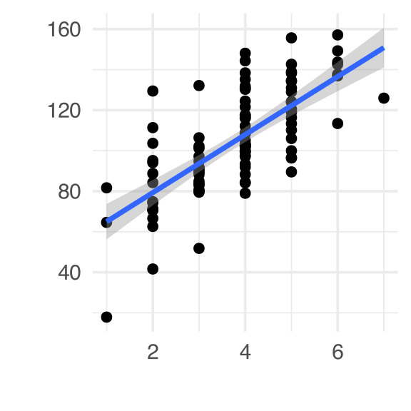
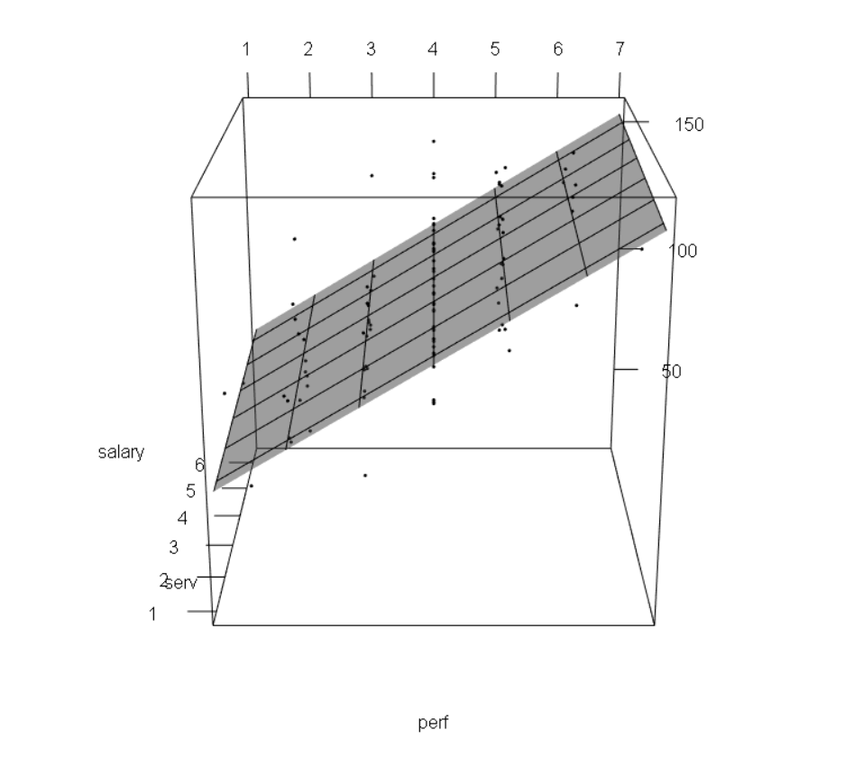
A linear model with two continuous predictors: three-dimensional plane!
Example: lm with 2 Predictors
Imagine we extend our study of test scores
We sample 150 students taking a multiple choice Biology exam (max score 40)
We give all students a survey at the start of the year measuring their school motivation
- We standardise this variable so the mean is 0, negative numbers are low motivation, and positive numbers high motivation
We then measure the hours they spent studying for the test, and record their scores on the test
Data
Mathematical model specification and lm code
\[\text{Score}_i = \color{blue}{\beta_0} + \color{blue}{\beta_1} \cdot \color{orange}{\text{Hours}_{i}} + \color{blue}{\beta_2} \cdot \color{orange}{\text{Motivation}_{i}} + \color{blue}{\epsilon_i}\]
parameters of the linear model (coefficients)
values we provide (inputs)
Multiple predictors are separated by + in the model specification:
Identifying coefficients from model summary
\[\text{Score}_i = \color{blue}{\beta_0} + \color{blue}{\beta_1} \cdot \color{orange}{\text{Hours}_{i}} + \color{blue}{\beta_2} \cdot \color{orange}{\text{Motivation}_{i}} + \color{blue}{\epsilon_i}\]
Call:
lm(formula = score ~ hours + motivation, data = test_study2)

Residuals:
     Min       1Q   Median       3Q      Max
-12.9548  -2.8042  -0.2847   2.9344  13.8240

Coefficients:
            Estimate Std. Error t value Pr(>|t|)
(Intercept)  6.86679    0.65473  10.488   <2e-16 ***
hours        1.37570    0.07989  17.220   <2e-16 ***
motivation   0.91634    0.38376   2.388   0.0182 *
---
Signif. codes:  0 '***' 0.001 '**' 0.01 '*' 0.05 '.' 0.1 ' ' 1

Residual standard error: 4.386 on 147 degrees of freedom
Multiple R-squared:  0.6696,    Adjusted R-squared:  0.6651
F-statistic: 148.9 on 2 and 147 DF,  p-value: < 2.2e-16
\(\color{blue}{\beta_0} = 6.87\)
\(\color{blue}{\beta_1} = 1.38\)
\(\color{blue}{\beta_2} = 0.92\)
Multiple Regression Coefficients
            Estimate Std. Error t value Pr(>|t|)
(Intercept)     6.87       0.65   10.49     0.00
hours           1.38       0.08   17.22     0.00
motivation      0.92       0.38    2.39     0.02
What is the interpretation (i.e., the meaning) of the…
intercept coefficient?
- A student who did not study, and who has average school motivation would be expected to score 6.87 on the test
slope over hours?
- Controlling for students’ level of motivation [or: Holding motivation level constant], for every additional hour studied, there is a 1.38 points increase in test score
slope over motivation?
- Controlling for hours of study [or: Holding hours of study constant], for every SD unit increase in motivation, there is a 0.92 points increase in test score
Using the model for prediction
Predicting (in this case, reconstructing) the score of individual ID101:
\(\color{blue}{\beta_0} = 6.87\)
\(\color{blue}{\beta_1} = 1.38\)
\(\color{blue}{\beta_2} = 0.92\)
\(\color{orange}{y} = 7\)
\(\color{orange}{x_1} = 2\)
\(\color{orange}{x_2} = -1.42\)
\[ \begin{align} \text{Score}_{ID101} &= \color{blue}{\beta_0} + \color{blue}{\beta_1} \cdot \color{orange}{\text{Hours}_{ID101}} + \color{blue}{\beta_2} \cdot \color{orange}{\text{Motivation}_{ID101}} + \color{blue}{\epsilon_{ID101}} \\ &= 6.87 + (1.38 \times 2) + (0.92 \times -1.42) + (-1.32) \\ &= 6.87 + 2.76 - 1.31 -1.32 \\ &= 7 \end{align} \]
Summary
- We run linear models using
lm()in R
- The intercept is the value of \(Y\) when \(X\) = 0
- The slope is the unit change in \(Y\) for each unit change in \(X\)
- In certain cases, we may standardise our variables; this will affect their interpretation
- We can easily add more predictors to our model
- When we do, our interpretations of the coefficients are when all other predictors are held constant
Back matter
This week
Tasks:
 Work on exercises in labs
 Complete the weekly quiz
Get support:
 Consult the flash cards
 Ask questions anonymously on Piazza
 We really like seeing you in office hours!