Introduction to linear regression

Data Analysis for Psychology in R 2

Dr. Patrick Sturt (Patrick.Sturt@ed.ac.uk)

Department of Psychology
University of Edinburgh
2026–2027

Course overview

Introduction to linear models (with Dr. Patrick Sturt)	Introduction to linear regression
	Interpreting linear models
	Testing predictors and evaluating linear models
	F-tests and model comparison
	Practice analysis: Linear models
Extending linear models (with Dr. Elizabeth Pankratz)	Categorical predictors and treatment coding
	Sum coding
	Assumptions and diagnostics
	Bootstrapping and confidence intervals
	Practice analysis: Categorical predictors (led by Patrick)

Interactions (with Dr. Elizabeth Pankratz)	Mean-centering and numeric/categorical interactions
	Numeric/numeric interactions
	Categorical/categorical interactions
	Testing simple effects and correcting for multiple comparisons
	Practice analysis: Interactions (led by Patrick)
Logistic regression (with Dr. Elizabeth Pankratz)	Probabilities and log-odds
	Modelling binary outcomes with logistic regression
	Interactions, assumptions, diagnostics, comparisons
	Practice analysis: Logistic regression (led by Patrick)
	Report feedback, exam prep, full-course Q&A

This Week’s Learning Objectives

1. Understand the link between models and functions

2. Understand the key concepts (intercept and slope) of the linear model

3. Understand what residuals represent

4. Understand the key principles of least squares

5. Be able to specify a simple linear model (labs)

Part 1: Functions & Models

What is a Model?

• Pretty much all statistics is about models

• A model is a formal representation of a system

• Put another way, a model is an idea about the way the world is

A Model as a Function

• We tend to represent mathematical models as functions

  • A function is an expression that defines the relationship between one variable (or set of variables) and another variable (or set of variables)

  • It allows us to specify what is important (arguments) and how these things interact with each other (operations)

• This allows us to make and test predictions

Example

• To think through these relations, we can use a simpler example

• Suppose I have a model for how long a baby’s body is, depending on how old the baby is:

\[ \text{Length} = 55 + 4 \times \text{Age} \]

• Length is measured in cm; Age is measured in months

• I’m using this model to formally represent the relationship between a baby’s age and their length

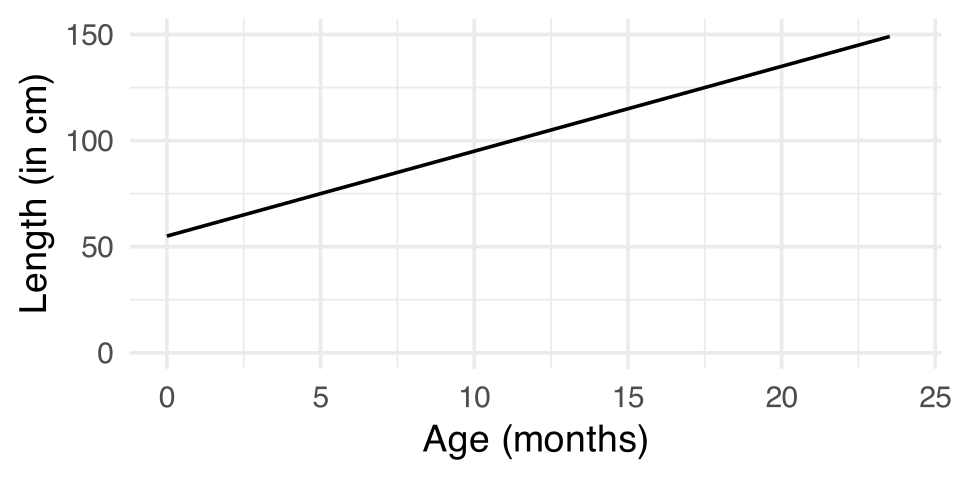
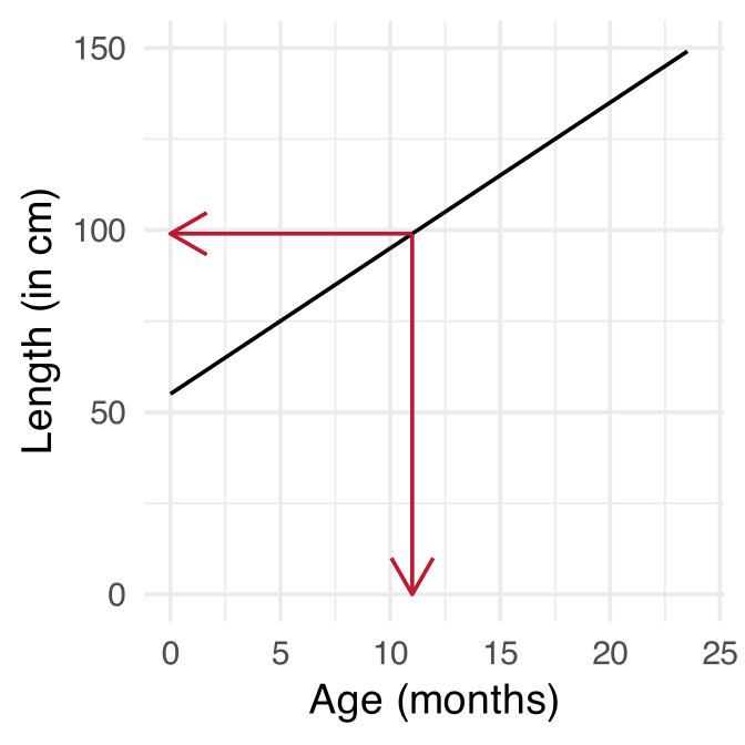
Visualising a Model

• The x-axis shows Age

• The y-axis shows Length

• The black line represents our model: \(y = 55+4x\)

Models as “a State of the World”

• Let’s suppose my model is true
  • That is, it is a perfect representation of how babies grow
• What are the implications of this?
  • My models creates predictions
    
  • IF my model is a true representation of the world, THEN data from the world should closely match my predictions

Predictions and Data

Age	PredictedLength
10.00	95
10.25	96
10.50	97
10.75	98
11.00	99
11.25	100
11.50	101

• Our predictions are points which fall on our line (representing the model, as a function)
• The arrows are showing how we can use the model to find a predicted value

Predictions and Data

• Consider the predictions when the children get a lot older…

• What does this say about our model?

• If we were to collect actual data on height and age, will our observations fall on the line?

Age	Year	Prediction_cm	Prediction_m
216	18	919	9.19
228	19	967	9.67
240	20	1015	10.15
252	21	1063	10.63
264	22	1111	11.11
276	23	1159	11.59
288	24	1207	12.07
300	25	1255	12.55

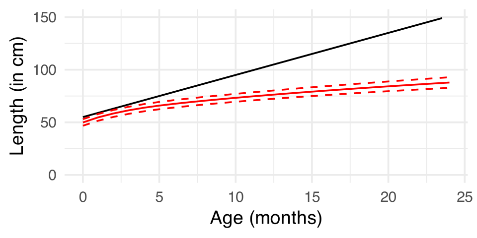
Length & Age is Non-Linear

• Our red line is plotted based on the mean length for different ages using real data

How can we judge how good the model is?

• We represent the model as a function. For linear regression models, that function is a line.

• The model yields predictions: values we expect if our model is true.

• We can collect data and see if the model’s predictions match the observed data.

• If they deviate, then that suggests our model is not so good.

Deterministic vs Statistical Models

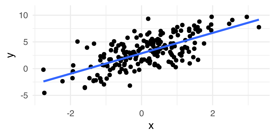
A deterministic model is a model for an exact relationship:

\[ y = \underbrace{3 + 2 x}_{f(x)} \]

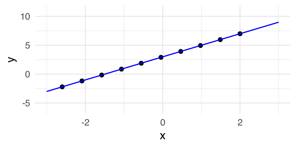
A statistical model allows for case-by-case variability:

\[ y = \underbrace{3 + 2 x}_{f(x)} + \epsilon \]

Part 2 & 3: Linear Model - Intercept, Slope, and Residuals

Linear Model

• Our focus in DAPR2 is on the linear model:

  • Assumes the relationship between the outcome variable and the predictor(s) is linear

  • Describes an outcome variable as a function of one or more predictor variables

  • In Blocks 1–3, we’ll look at continuous numeric outcome variables; in Block 4, we’ll learn how to deal with binary outcome variables (e.g., yes/no, correct/incorrect)

Example

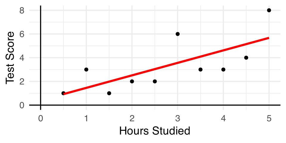
Question: Do students who study more get higher scores on the test?

student	hours	score
ID1	0.5	1
ID2	1.0	3
ID3	1.5	1
ID4	2.0	2
ID5	2.5	2
ID6	3.0	6
ID7	3.5	3
ID8	4.0	3
ID9	4.5	4
ID10	5.0	8

Codebook

• student = ID variable unique to each respondent

• hours = the number of hours spent studying. This will be our predictor (\(x\))

• score = test score. This will be our outcome (\(y\))

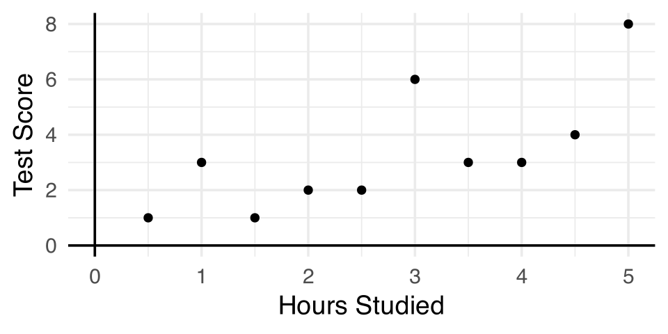
Scatterplot of Data

The best linear model of the data

Definition of the Line

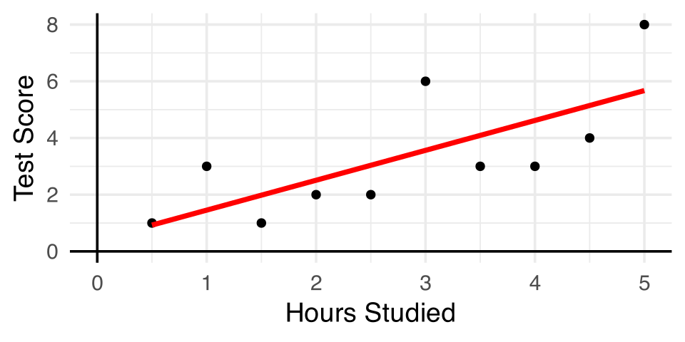
• The line can be described by two values, called “parameters”:

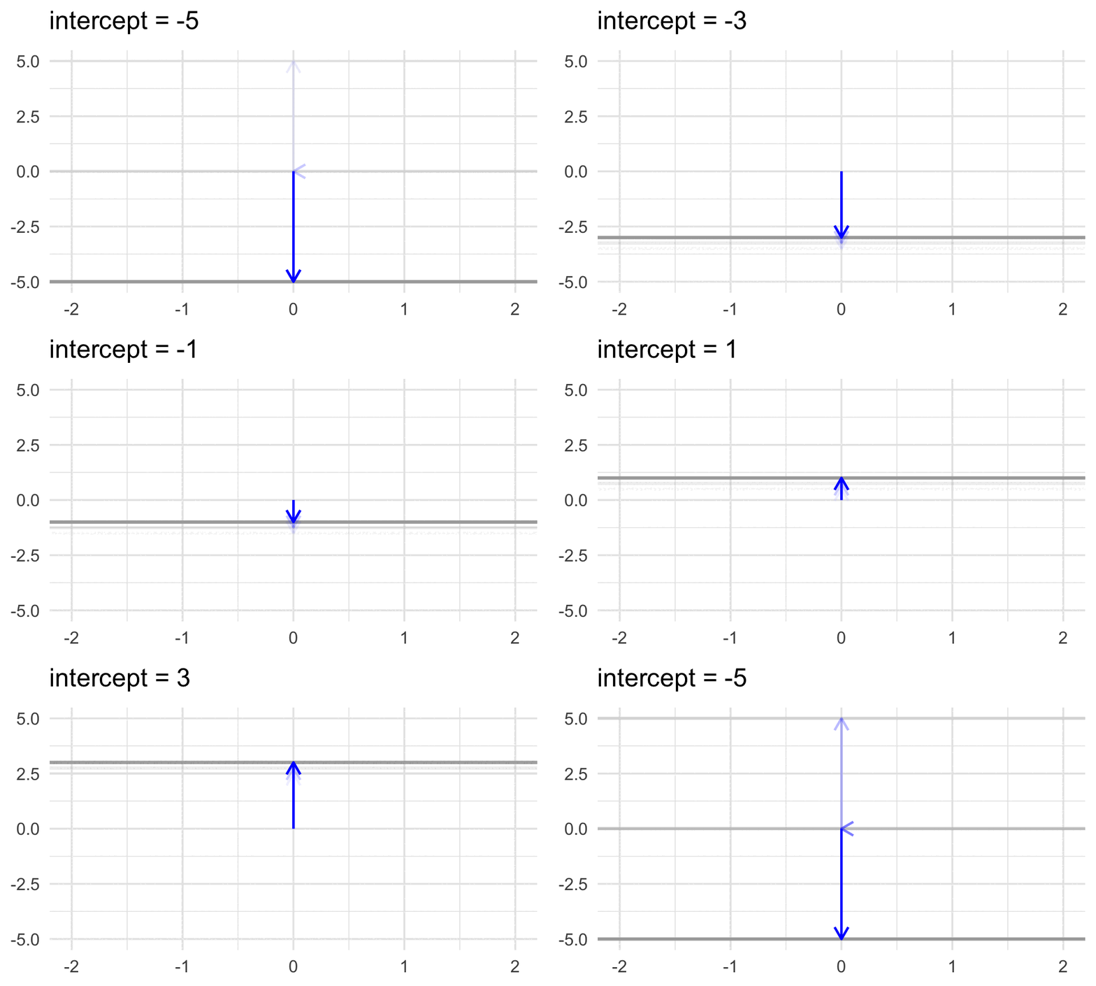
  • Intercept: the point where the line crosses (or “intercepts”) the \(y\)-axis, or in other words, the point where \(x = 0\)

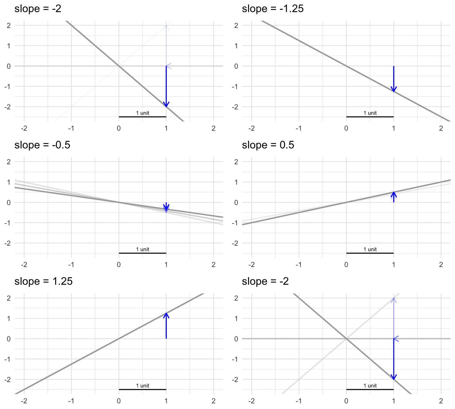
  • Slope: the gradient of the line, or rate of change

Intercept and Slope

• height of the line (intercept)

• gradient of the line (slope)

Linear Model Equation

\[y_i = \beta_0 + \beta_1 x_{i} + \epsilon_i\]

• \(y_i\) = the outcome variable (e.g. score)

• \(x_i\) = the predictor variable, (e.g. hours)

• \(\beta_0\) = intercept

• \(\beta_1\) = slope

• \(\epsilon_i\) = residual (we will come to this shortly)

Linear Model Equation

\[y_i = \beta_0 + \beta_1 x_{i} + \epsilon_i\]

• Why do we have \(i\) in some places and not others?

• \(i\) is a subscript to indicate that each participant has their own value.

• So each participant has their own:

  • score on the test ( \(y_i\) )
  • number of hours studied ( \(x_i\) ) and
  • residual term ( \(\epsilon_i\) )

• What does it mean that the intercept ( \(\beta_0\) ) and slope ( \(\beta_1\) ) do not have the subscript \(i\)?

• It means there is one value for all observations.
  • Remember the model is for all of our data

What is \(\epsilon_i\)?

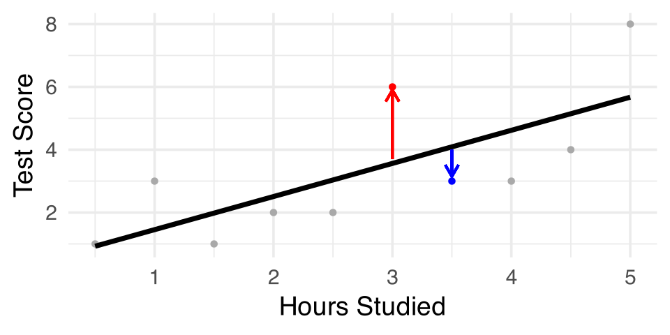
• The vertical distance between the model-predicted line and a data point.
  • \(\epsilon_i\) is positive if the point is above the line (red in plot)
  • \(\epsilon_i\) is negative if the point is below the line (blue in plot)

How to Find the Line?

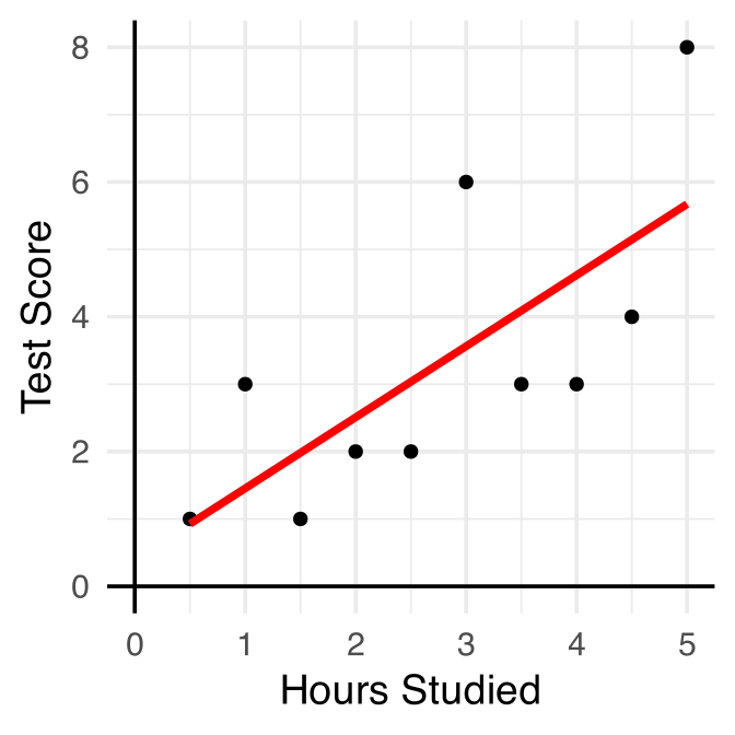
• The line represents a model of our data.

  • In our example, the model that best characterises the relationship between hours of study and test score

• In the scatterplot, the data are represented by points

• So a good line is a line that is “close” to all points

• The method that we use to identify the best-fitting line is the Principle of Least Squares

Part 4: Principle of Least Squares

Linear Model

• So far we have introduced the linear model:

\[y_i = \beta_0 + \beta_1 x_{i} + \epsilon_i\]

• Where

  • \(y_i\) is our measured outcome variable
  • \(x_i\) is our measured predictor variable
  • \(\beta_0\) is the model intercept
  • \(\beta_1\) is the model slope
  • \(\epsilon_i\) is the residual error (difference between the model predicted and the observed value of \(y\))

How do we calculate \(\beta_0\) and \(\beta_1\)?

Principle of Least Squares

• The values \(\beta_0\) and \(\beta_1\) are typically unknown and need to be estimated from our data.

  • We denote the “best” estimated values as \(\hat \beta_0\) and \(\hat \beta_1\)

• We find the values of \(\hat \beta_0\) and \(\hat \beta_1\) (and thus our best line) using least squares

• Least squares:

  • minimises the distances between the actual values of \(y\) and the model-predicted values of \(\hat y\)

  • that is, it minimises the residuals for each data point (the line is “close” to the data points)

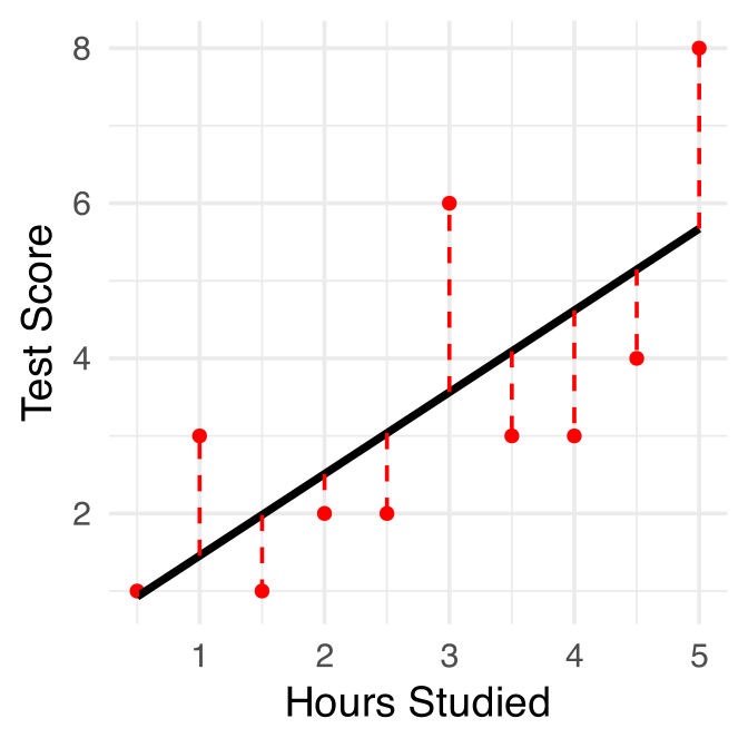
Least Squares step-by-step (1)

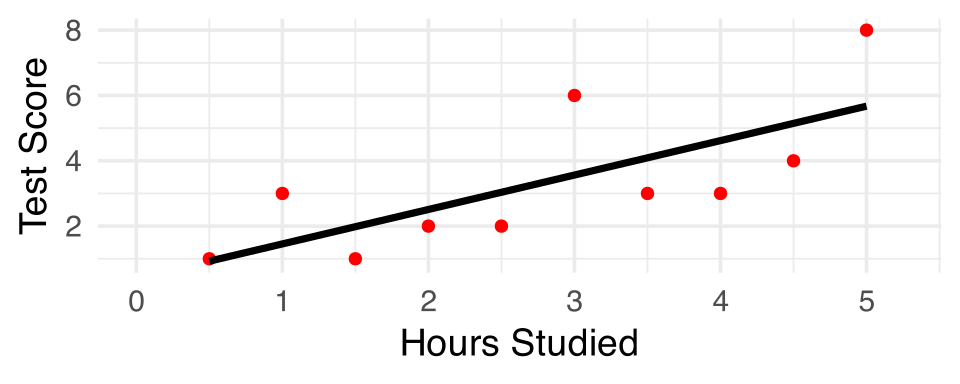
• Define some line

Least Squares step-by-step (2)

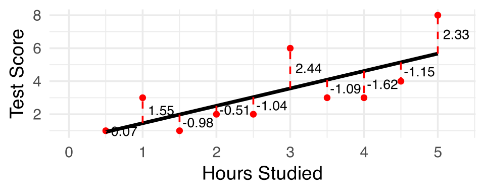
• Define some line
• Calculate the residuals

Least Squares step-by-step (3)

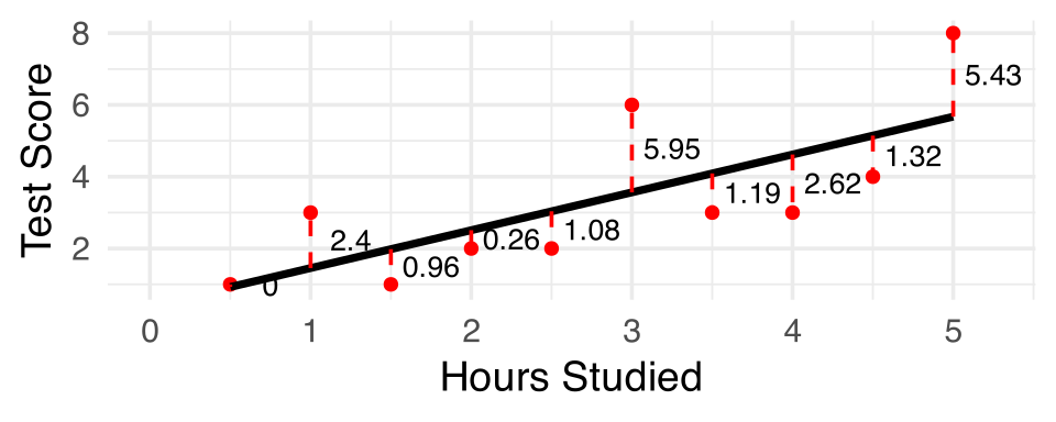
• Define some line
• Calculate the residuals
• Square them

Least Squares step-by-step (4)

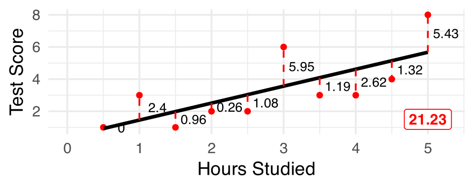
• Define some line
• Calculate the residuals
• Square them
• Sum up the squares

The best line is the one that minimises the residual sum of squares.

Why do you think we square the residuals?

Residual Sum of Squares

\[SS_{Residual} = \sum_{i=1}^{n}(y_i - \hat{y}_i)^2\]

Residual Sum of Squares

\[SS_{Residual} = \sum_{i=1}^{n}(\color{#BF1932}{y_i} - \hat{y}_i)^2\]

• Data = \(y_i\)
  • This is what we have measured in our study
  • For us, the test scores

Residual Sum of Squares

\[SS_{Residual} = \sum_{i=1}^{n}(y_i - \color{#BF1932}{\hat{y}_i})^2\]

• Data = \(y_i\)
  • This is what we have measured in our study
  • For us, the test scores

• Predicted value = \(\hat{y}_i = \hat \beta_0 + \hat \beta_1 x_i\)
  • Or, the value of the outcome our model predicts given someone’s values for predictors
    
  • In our example: given you study for 4 hours, what test score does our model predict you will get?

Residual Sum of Squares

\[SS_{Residual} = \sum_{i=1}^{n}(\color{#BF1932}{y_i - \hat{y}_i})^2\]

• Data = \(y_i\)
  • This is what we have measured in our study
    
  • For us, the test scores.
• Predicted value = \(\hat{y}_i = \hat \beta_0 + \hat \beta_1 x_i\)
  • Or, the value of the outcome our model predicts given someone’s values for predictors
    
  • In our example: given you study for 4 hours, what test score does our model predict you will get?

• Residual = Difference between \(y_i\) and \(\hat{y}_i\)

Key Point

• It is worth a brief pause as this is a very important point

The values of the intercept and slope that minimise the sum of square residual are our estimated coefficients from our data

Minimising the \(SS_{residual}\) means that across all our data, the predicted values from our model are as close as they can be to the actual measured values of the outcome

Calculating the Slope

\[\hat \beta_1 = \frac{SP_{xy}}{SS_x}\]

• \(SP_{xy}\) = sum of cross-products:

\[SP_{xy} = \sum_{i=1}^{n}(x_i - \bar{x})(y_i - \bar{y})\]

• \(SS_x\) = sums of squared deviations of \(x\):

\[SS_x = \sum_{i=1}^{n}(x_i - \bar{x})^2\]

• Where:
  • \(x_i\) = predictor data (in our example, hours)
  • \(y_i\) = outcome data (in our example, scores)
  • \(\bar{y}\) = mean of \(y\)
  • \(\bar{x}\) = mean of \(x\)
  • \(n\) = total number of observations
  • \(\Sigma\) = sum it all up

Calculating the Intercept

\[\hat \beta_0 = \bar{y} - \hat \beta_1 \bar{x}\]

• Where:
  • \(\hat \beta_1\) = slope estimate
  • \(\bar{y}\) = mean of \(y\)
  • \(\bar{x}\) = mean of \(x\)

Part 5: Simple Linear Model in R

Understanding the Linear Model Equation

\[\hat{y}_i = \color{blue}{b_0 \cdot{}}\color{orange}{1} \color{blue}{+b_1 \cdot{}} \color{orange}{x_i}\]

• values of the linear model (coefficients)

• values we provide (inputs)

• maps directly to R “formula” notation y ~ 1 + x

lm in R

• In R, we use the lm() function

lm(DV ~ IV, data = datasetName)

• The first bit of code is the model formula:
  • The outcome or DV appears on the left of ~
  • The predictor(s) or IV appear on the right of ~
• We then give R the name of the data set
  • This set must contain variables (columns) with the same names as you have specified in the model formula

lm in R

• First need some data:

test <- tibble(
  student = paste(rep("ID",10),1:10, sep=""),
  hours = seq(0.5,5,.5),
  score = c(1,3,1,2,2,6,3,3,4,8)
)

• Look at first few rows:

head(test, 4)

# A tibble: 4 x 3
  student hours score
  <chr>   <dbl> <dbl>
1 ID1       0.5     1
2 ID2       1       3
3 ID3       1.5     1
4 ID4       2       2

lm in R

• Build and run model in R, store in object named mod1:

mod1 <- lm(score ~ hours, data = test)

mod1

Call:
lm(formula = score ~ hours, data = test)

Coefficients:
(Intercept)        hours  
      0.400        1.055  

lm in R

• Look at summary() of output in R:

summary(mod1)

Call:
lm(formula = score ~ hours, data = test)

Residuals:
    Min      1Q  Median      3Q     Max 
-1.6182 -1.0773 -0.7454  1.1773  2.4364 

Coefficients:
            Estimate Std. Error t value Pr(>|t|)  
(Intercept)   0.4000     1.1111   0.360   0.7282  
hours         1.0545     0.3581   2.945   0.0186 *
---
Signif. codes:  0 '***' 0.001 '**' 0.01 '*' 0.05 '.' 0.1 ' ' 1

Residual standard error: 1.626 on 8 degrees of freedom
Multiple R-squared:  0.5201,    Adjusted R-squared:  0.4601 
F-statistic:  8.67 on 1 and 8 DF,  p-value: 0.01858

Summary

• In statistics, we are building models that describe how a set of variables relate
• The linear model describes our data based on an intercept and a slope(s)
• From this model (line) we can make predictions about peoples scores on an outcome
• The degree to which our predictions differ from the observed data = residual = error = how good (or bad) the model is
• We find our model coefficients based on least squares, which are the coefficients that minimise the sum of squared residuals

This week

Tasks:

Work on exercises in labs

Complete the weekly quiz

Get support:

Consult the flash cards

Ask questions anonymously on Piazza

We really like seeing you in office hours!