
Manual contrast interactions and multiple comparisons
Data Analysis for Psychology in R 2
Where we are in the analysis workflow

Today’s data
The subjective wellbeing (SWB) of patients at two different hospitals:
Hosp1:

Hosp2:

who have undergone one of three different treatments for depression:
Cognitive Behavioural Therapy (CBT)

Eye Movement Desensitisation and Reprocessing therapy (EMDR)

Antidepressant medication
(Meds):

Visualising the interaction we’ll test
We want to know: Is there a difference between hospitals in how different treatment types (talk therapy vs. pharmaceutical therapy) are associated with SWB?

Step 1: Define means of all combinations of factor levels
When we test differences between groups, we’re testing differences between group means.
So, we will start by defining the group means for all combinations of factor levels in our data.
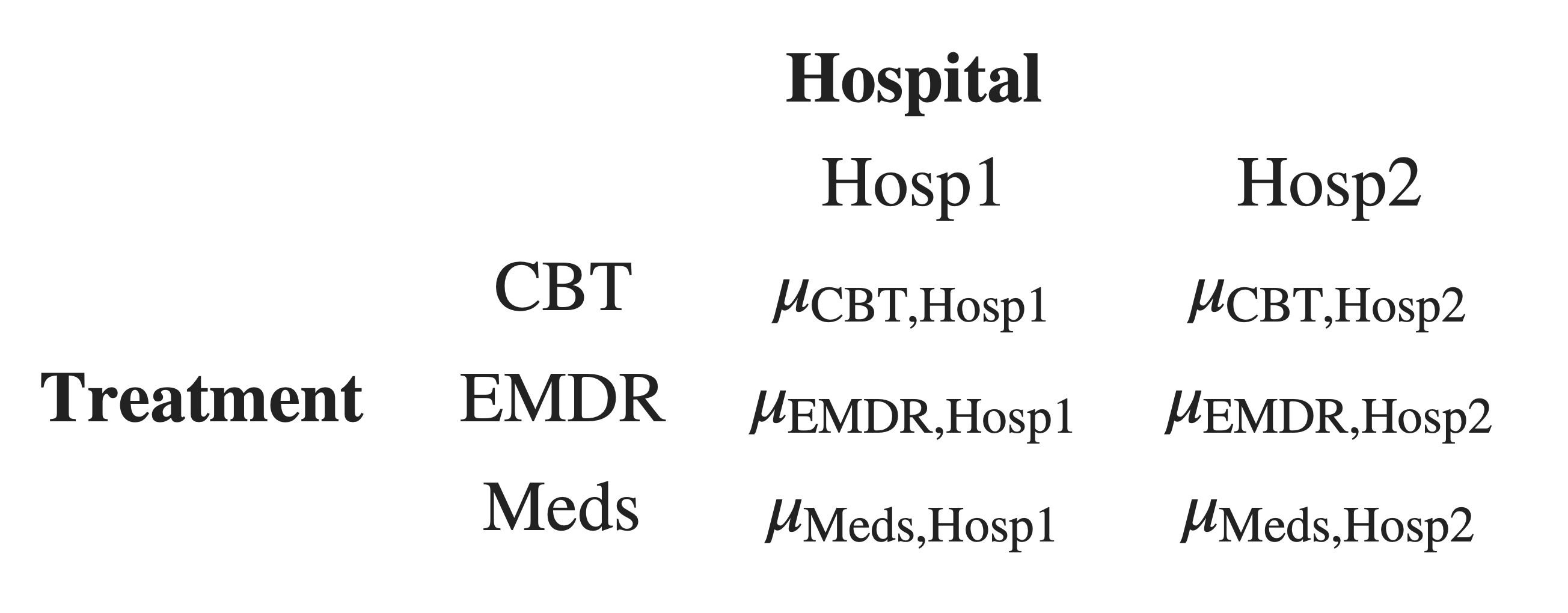
Next, we’ll combine these group means in the way that the manual contrasts specify.
Step 2: “Chunk” some of the means together
Within each hospital, we chunk CBT and EMDR together, because they are both talk therapy.
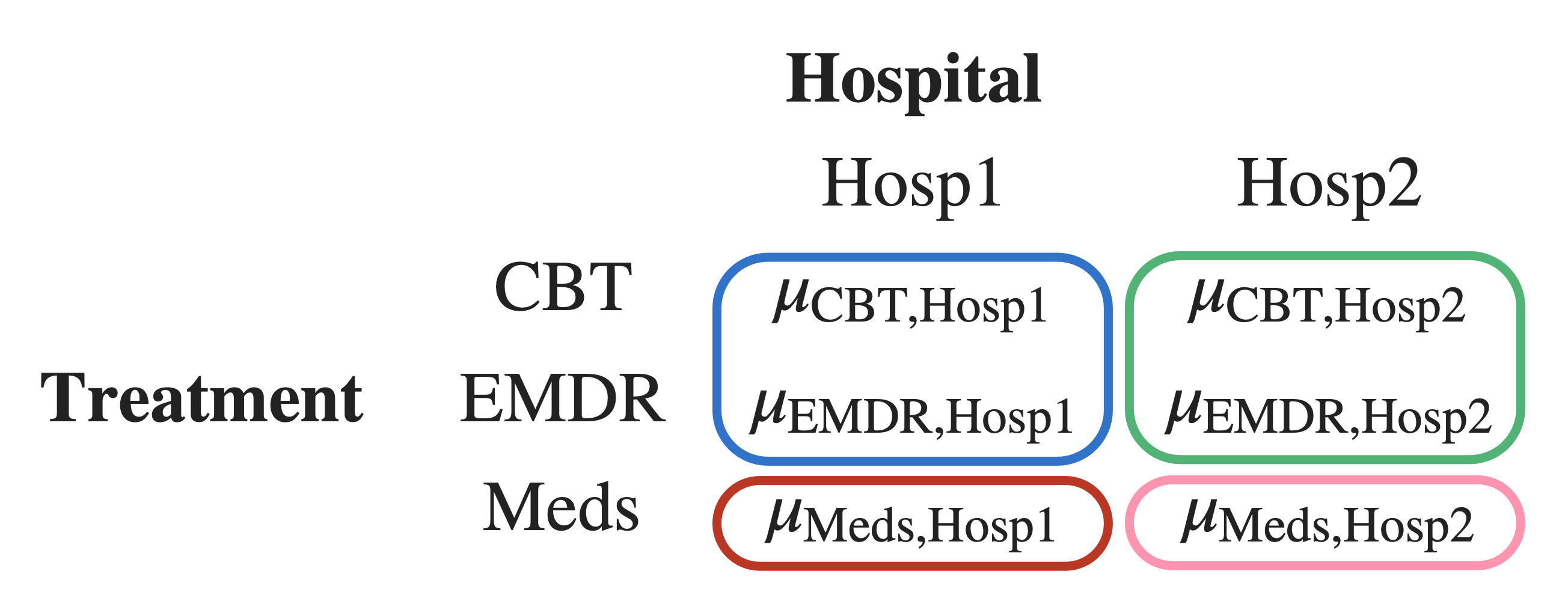
When we chunk two group means together, mathematically we are taking the mean of those group means.
To represent the mean of the blue chunk (top left):
\[ \frac{ \mu_{\text{CBT,Hosp1}} + \mu_{\text{EMDR,Hosp1}} }{2} \]
To represent the mean of the green chunk (top right):
\[ \frac{ \mu_{\text{CBT,Hosp2}} + \mu_{\text{EMDR,Hosp2}} }{2} \]
Test the interaction contrast
When we test the contrast using contrast(), we are testing the H0 that the estimate is equal to zero. For this interaction, the H0 says there’s no difference between Hospital in how TrtmtType is associated with SWB.
(m1_ixn_test <- contrast(m1_emm, interaction_contr)) contrast estimate SE df t.ratio p.value
TrtmtType:Hospital -3.73 0.641 174 -5.819 <0.0001Get the associated 95% CIs using confint():
(m1_ixn_confint <- confint(m1_ixn_test)) contrast estimate SE df lower.CL upper.CL
TrtmtType:Hospital -3.73 0.641 174 -4.99 -2.46
Confidence level used: 0.95 The null hypothesis:
- There’s no difference between hospitals in how different treatment types (talk therapy vs. pharmaceutical therapy) are associated with SWB.
- In other words, if the null hypothesis were true, the data for both hospitals would pattern the same.
Can we reject the null hypothesis?
![]()
![]()
Extending the analysis workflow

 Retrieval practice: Testing simple effects
- What’s a simple effect?
- If I ask for simple effects of
Hospitalat each level ofTreatment, what am I looking for? - What’s the difference between simple effects and simple slopes?
- What does it mean to test a simple effect?
Simple effects of Hospital at each level of Treatment
pairs(m1_emm, simple = "Hospital")Treatment = CBT:
contrast estimate SE df t.ratio p.value
Hosp1 - Hosp2 2.12 0.523 174 4.059 <0.0001
Treatment = EMDR:
contrast estimate SE df t.ratio p.value
Hosp1 - Hosp2 -3.69 0.523 174 -7.047 <0.0001
Treatment = Meds:
contrast estimate SE df t.ratio p.value
Hosp1 - Hosp2 2.95 0.523 174 5.632 <0.0001
Note on the positive/negative signs:
pairs()computesHosp1 – Hosp2because of how factor levels in the factorHospitalare ordered.- To compute
Hosp2 – Hosp1instead, we would have to codeHosp2as the reference level ofHospitalbefore fitting the model.
Simple effects of Treatment for each level of Hospital
pairs(m1_emm, simple = "Treatment")Hospital = Hosp1:
contrast estimate SE df t.ratio p.value
CBT - EMDR 0.673 0.523 174 1.287 0.4044
CBT - Meds -0.697 0.523 174 -1.332 0.3796
EMDR - Meds -1.370 0.523 174 -2.619 0.0259
Hospital = Hosp2:
contrast estimate SE df t.ratio p.value
CBT - EMDR -5.137 0.523 174 -9.819 <0.0001
CBT - Meds 0.127 0.523 174 0.242 0.9682
EMDR - Meds 5.263 0.523 174 10.061 <0.0001
P value adjustment: tukey method for comparing a family of 3 estimates 
What’s this “P value adjustment: tukey method” thing? We’ll find out soon, but first …
Visualising cat/cat interactions
Using cat_plot():
interactions::cat_plot(
  m1,
  pred = Hospital,
  modx = Treatment,
  geom = 'line'
)
Using emmip() (estimated marginal means interaction plot):
emmip(
  m1_emm,
  Treatment ~ Hospital,
  CIs = TRUE
)
Let’s roll some dice
On a twenty-sided die (a d20), the probability of rolling a 1 (or any other individual number) is 1/20 = 5%.
But if we roll the d20 over and over again, the probability that we’ll roll a 1 at least once goes up and up and up.

\(.05\)
\(= 1 – 0.95\)
\(.0975\)
\(= 1 – (0.95 \times 0.95)\)
\(.1426\)
\(= 1 – (0.95 \times 0.95 \times 0.95) = 1 - 0.95^3\)
In general:
\[ P(\text{rolling a 1 in m rolls}) = 1 - (1 - 0.05)^m \]
What’s the probability that we’ll roll a 1 at least once in twenty rolls?
wooclap.com, code UBEQCF
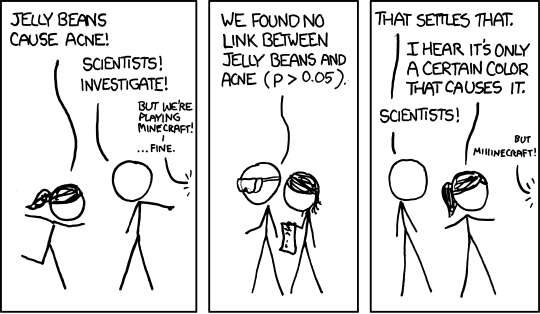
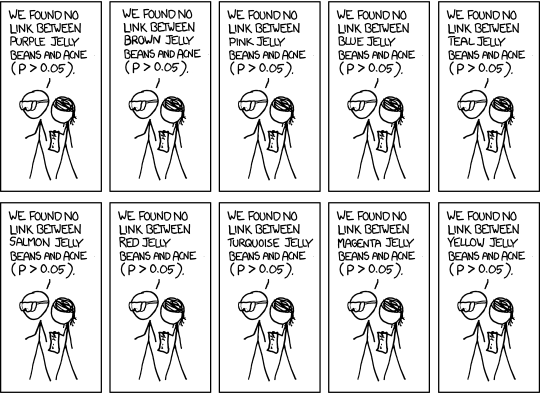
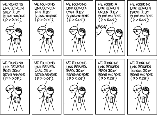
relevant XKCD (https://xkcd.com/882/)

Analysis workflow: The final form!

This week
Tasks:

Attend your lab and work together on the exercises
Support:

Help each other on the Piazza forum

Complete the weekly quiz

Attend office hours (see Learn page for details)
Code for data plot
hosp |>
  ggplot(aes(x = Treatment, y = SWB, colour = Treatment, fill = Treatment)) +
  geom_violin(alpha = 0.5) +
  geom_jitter(alpha = 0.5, size = 5) +
  facet_wrap(~ Hospital) +
  stat_summary(fun = mean, geom = 'point', colour = 'black', size = 8, show.legend = F) +
  theme(legend.position = 'none') +
  NULL
Code for visualising manual chunks
hosp |>
  mutate(
    TrtmtType = ifelse(Treatment == 'Meds', 'PharmaTherapy', 'TalkTherapy')
  ) |>
  ggplot(aes(x = TrtmtType, y = SWB)) +
  geom_violin() +
  geom_jitter(aes(colour = Treatment), alpha = 0.5, size = 5) +
  facet_wrap(~ Hospital) +
  NULL