
Categorical predictors and dummy coding
Data Analysis for Psychology in R 2
 Warm-up activity: Line drawing
Draw each of the lines that’s defined by the given intercept and slope.
Line 1:
- Intercept is 0
- Slope is 1
Line 2:
- Intercept is 1
- Slope is –1

Line 3:
- Intercept is –1
- Slope is 2

Categorical predictors with two levels
aka binary predictors

Categorical predictors with two levels
aka binary predictors

Categorical predictors with two levels
aka binary predictors

But: linear models can only deal with input in number form.
So we need a way to represent the levels of these variables as numbers.
The way we’ll learn about today: dummy coding, aka treatment coding.
Dummy/treatment coding represents one level as 0, and the other level as 1
Schematic:

Studying
aloneis coded as 0.Studying with
othersis coded as 1.
In the data:
score_data |>
  select(ID, study, study_num) |>
  head(10)
ID study study_num
1 ID101 others 1
2 ID102 alone 0
3 ID103 alone 0
4 ID104 others 1
5 ID105 alone 0
6 ID106 others 1
7 ID107 alone 0
8 ID108 alone 0
9 ID109 others 1
10 ID110 alone 0Why does it matter which level is coded as 0
and which level is coded as 1?
To illustrate: Here are test scores from students who studied either alone (blue) or with others (pink).


Why does it matter which level is coded as 0
and which level is coded as 1?
A linear model will fit a line to this data.
Before I show you this line, I want you to make predictions about it.
 Predict individually: Write down your guesses:
- The line’s intercept will be the same as the mean of either alone or others. Which one? Why?
- Will the slope of the line be positive or negative? Why?
 Explain in pairs/threes: Why do you think your guesses are likely to be correct?

Visualising the model’s predictions


We have almost all the pieces!
But finding the SE for the non-reference level is mathematically a little complicated.
A nice shortcut: an R package called emmeans.
Plotting marginal means and CIs
emmeans has a built-in plot style.
plot(m1_emm) + coord_flip()
It’s OK, but a bit boring. We can definitely do better.
Plotting marginal means and CIs
# Save EMMs in tibble format,
# with compatible column names
m1_emm_df <- m1_emm |>
  as_tibble() |>
  rename(score = emmean)

# Plot the data like before,
# and now overlay EMMs
score_data |>
  ggplot(aes(x = study, y = score, fill = study, colour = study)) +
  geom_violin(alpha = 0.5) +
  geom_jitter(alpha = 0.5, width = 0.3, size = 5) +
  theme(legend.position = 'none') +
  scale_colour_manual(values = pal) +
  scale_fill_manual(values = pal) +
  geom_errorbar(
    data = m1_emm_df,
    aes(ymin = lower.CL, ymax = upper.CL),
    colour = 'black',
    width = 0.2,
    linewidth = 2
  ) +
  geom_point(
    data = m1_emm_df,
    colour = 'black',
    size = 5
  )
emmeans is an amazingly useful tool.
It can do LOTS more than we’ve seen here!
We’ll see more examples in the coming days and weeks.
Building an analysis workflow


Extension: Changing the reference level
If reference level = alone:

If reference level = others:

When others is the reference level (that is, the level represented as 0):
- What does the intercept represent?
- What does the slope represent?
- Why is the slope negative now, when before it was positive?
- Challenge: What hypotheses would a linear model test about this data?
Examples of categorical predictors with >2 levels
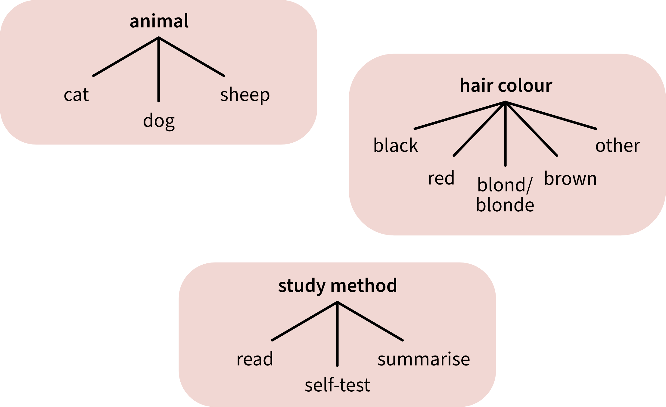
Today’s data: Study method


How do we fit a line to data from three groups?
- It’s impossible to draw one single straight line through all three group means.
- The smallest number of straight lines that connect all three group means is two.
- For this reason, we’re going to use two predictors. These two predictors are called “dummy variables”.
- In general, for a categorical predictor with \(k\) levels, we’ll use \(k-1\) dummy variables.
Dummy variables let us extend dummy/treatment coding to >2 levels

Both dummy variables have the same reference level: read.
- The first dummy variable will compare
self-testback toread. - The second dummy variable will compare
summariseback toread.
Dummy variables let us extend dummy/treatment coding to >2 levels
First dummy variable: self-test vs. read.

Second dummy variable: summarise vs. read.

- Is the slope of the first dummy variable positive or negative?


- Is the slope of the second dummy variable positive or negative?
- Is the slope of the first dummy variable bigger than the slope of the second dummy variable?
- Is the intercept of the first dummy variable bigger than the intercept of the second dummy variable?
How do we know that a model will use these particular dummy variables?
The function contrasts() shows us how a categorical predictor will be coded.
(You’ll get error messages if the variable is not stored as a factor.)
contrasts(score_data$method) self-test summarise
read 0 0
self-test 1 0
summarise 0 1How to read this output:
- Each column contains one dummy variable.
self-testcomparesself-test(the 1 in that column) toread.summarisecomparessummarise(the 1 in that column) toread.
- We know that the reference level is
readbecause in BOTH dummy variables,readis coded as 0.
 Now is a good time for questions!
What does each coefficient mean? (1)
Coefficients:
                 Estimate Std. Error t value Pr(>|t|)
 (Intercept)       23.414      0.866   27.03   <2e-16 ***
 methodself-test    4.162      1.319    3.16   0.0018 **
 methodsummarise    0.782      1.193    0.66   0.5127
(Intercept) aka \(\beta_0\): The mean score for the reference level (read).
mean_read[1] 23.4What hypothesis is the model testing here?
- Null hypothesis: The mean score for the reference level (
read) is equal to zero. - \(p\)-value: the probability of observing an intercept of 23.414, assuming that the true intercept is zero.
Can we reject this null hypothesis?
If we care about differences between study methods, is this null hypothesis interesting?
What does each coefficient mean? (2)
Coefficients:
                 Estimate Std. Error t value Pr(>|t|)
 (Intercept)       23.414      0.866   27.03   <2e-16 ***
 methodself-test    4.162      1.319    3.16   0.0018 **
 methodsummarise    0.782      1.193    0.66   0.5127
methodself-test aka \(\beta_1\): The difference between the mean score of self-test and the mean score of read.
mean_self - mean_read[1] 4.16What hypothesis is the model testing here?
- Null hypothesis: The difference between the mean score of
self-testand the mean score ofreadis equal to zero. - \(p\)-value: the probability of observing a difference of 4.162, assuming that the true difference is zero.
Can we reject this null hypothesis?
If we care about differences between study methods, is this null hypothesis interesting?
What does each coefficient mean? (3)
Coefficients:
                 Estimate Std. Error t value Pr(>|t|)
 (Intercept)       23.414      0.866   27.03   <2e-16 ***
 methodself-test    4.162      1.319    3.16   0.0018 **
 methodsummarise    0.782      1.193    0.66   0.5127
methodsummarise aka \(\beta_2\): The difference between the mean score of summarise and the mean score of read.
mean_summ - mean_read[1] 0.782What hypothesis is the model testing here?
- Null hypothesis: The difference between the mean score of
summariseand the mean score ofreadis equal to zero. - \(p\)-value: the probability of observing a difference of 0.782, assuming that the true difference is zero.
Can we reject this null hypothesis?
If we care about differences between study methods, is this null hypothesis interesting?
Now is a good time for questions!
Intro to testing hypotheses with emmeans
- Get estimated marginal means and 95% CIs for each level of the predictor. (This is as far as we got last time.)
(m2_emm <- emmeans(m2, ~method)) method emmean SE df lower.CL upper.CL
read 23.4 0.866 247 21.7 25.1
self-test 27.6 0.994 247 25.6 29.5
summarise 24.2 0.820 247 22.6 25.8
Confidence level used: 0.95 
When would you test your own contrasts using emmeans?
Testing our own contrasts using emmeans is not necessary for every analysis.
But it is useful if the hypotheses we want to test are not the same hypotheses that our a priori contrast coding (e.g., our dummy coding) will test.
Now is a good time for questions!
Changing the reference level
Another prediction activity:
Before, the reference level of method was read, and the non-reference levels were self-test and summarise.
Now, the reference level of method is summarise, and the non-reference levels are read and self-test.
- Would you expect the model coefficients to be the same or different?
- Would you expect the p-values of each model coefficient to be the same or different?
- Would you expect the estimated marginal means to be the same or different?
Predict: Write down your guesses about each question.
Explain: Why do you think your guesses are likely to be correct?
We’ll work through the example and you can check your predictions after.
Understanding the new dummy variables
First new dummy variable:
read vs. summarise.

Second new dummy variable:
self-test vs. summarise.

- Is the slope of the first dummy variable positive or negative?
- Is the slope of the second dummy variable positive or negative?
- Will the coefficient estimates be the same or different compared to our previous model?
Changing the reference level: emmeans
m3_emm <- emmeans(m3, ~method)Reference level = summmarise (new).
plot(m3_emm) + coord_flip()
Reference level = read (old).
plot(m2_emm) + coord_flip()
Are the estimated marginal means and 95% CIs from each model the same or different?
What difference does it make to change the reference level?
When the reference level of method is summarise, instead of read:
- The model coefficients are different.
- The set of hypotheses that the model tests are different.
- The estimated marginal means are the same.
Observe: Did your guesses match these results?
Explain: Why are the results the way they are?
Building an analysis workflow
This week
Tasks

Attend your lab and work together on the exercises
Support

Help each other on the Piazza forum

Complete the weekly quiz

Attend office hours (see Learn page for details)
Why does it matter which level is coded as 0
and which level is coded as 1?
Predict individually: Write down your guesses:
- The line’s intercept will be the same as the mean of either alone or others. Which one? Why?
- Will the slope of the line be positive or negative? Why?
Explain in pairs/threes: Why do you think your guesses are likely to be correct?
Observe: Did your guesses match these results?
Explain: Why are the results the way they are?

How do we describe this line?
Using our mathematical toolkit:
\[ \text{score}_i = \beta_0 + (\beta_1 \cdot \text{study}) + \epsilon_i \]
\(\beta_0\): intercept, mean of alone (the level coded as 0):
mean_alone[1] 22.8\(\beta_1\): slope, the difference between mean of others (coded as 1) and mean of alone (coded as 0):
mean_others - mean_alone[1] 4.73\(\epsilon_i\): error for each individual data point \(i\)

