Testing and Evaluating LM

Data Analysis for Psychology in R 2

Emma Waterston

Department of Psychology
University of Edinburgh
2025–2026

Course Overview

Introduction to Linear Models	Intro to Linear Regression
	Interpreting Linear Models
	Testing Individual Predictors
	Model Testing & Comparison
	Linear Model Analysis
Analysing Experimental Studies	Categorical Predictors & Dummy Coding
	Effects Coding & Coding Specific Contrasts
	Assumptions & Diagnostics
	Bootstrapping
	Categorical Predictor Analysis

Interactions	Interactions I
	Interactions II
	Interactions III
	Analysing Experiments
	Interaction Analysis
Advanced Topics	Power Analysis
	Binary Logistic Regression I
	Binary Logistic Regression II
	Logistic Regression Analysis
	Exam Prep and Course Q&A

This Week’s Learning Objectives

1. Understand how to interpret significance tests for \(\beta\) coefficients

2. Understand how to calculate and interpret \(R^2\) and adjusted- \(R^2\) as a measure of model quality

3. Be able to locate information on the significance of individual predictors and overall model fit in R lm model output

Part 1: Recap & Overview

Recap

• Last week we expanded the general linear model equation to include multiple predictors:

\[ y_i = \beta_0 + \beta_1 \cdot x_{1i} + \beta_2 \cdot x_{2i} + \beta_j \cdot x_{ji} + \epsilon_i \]

• And we ran an example concerning test scores:

\[ \text{Score}_i = \beta_0 + \beta_1 \cdot \text{Hours}_{i} + \beta_2 \cdot \text{Motivation}_{i} + \epsilon_i \]

• And we looked at how to run this model in R:

lm(score ~ hours + motivation, data = test_study2)

Evaluating our Model

So far we have estimated values for the key parameters of our model ( \(\beta\)s )

• Now we have to think about how we evaluate the model

• Evaluating a model will consist of:

  1. Evaluating the individual coefficients

  2. Evaluating the overall model quality

  3. Evaluating the model assumptions

Important: Before accepting a set of results, all three of these aspects of evaluation must be considered

• We will talk about evaluating individual coefficients and model quality today
• Model assumptions covered later in the course (Semester 1, Week 8)

Significance of Individual Effects

• A general way to ask this question would be to state:

Is our model informative about the association between X and Y?

• In the context of our example from last lecture, we could ask,

Is study time a useful predictor of test score?

• The above is a research question

• We need to turn this into a testable statistical hypothesis

Evaluating Individual Predictors

Steps in hypothesis testing:

• Research question

• Statistical hypothesis

• Define the null hypothesis

• Calculate an estimate of effect of interest

• Calculate an appropriate test statistic

• Evaluate the test statistic against the null

Research Questions and Hypotheses

Research questions are statements of what we intend to study

• A good question defines:

• constructs under study
• the association being tested
• a direction of association
• target populations etc.

Does increased study time improve test scores in school-age children?

Research Questions and Hypotheses

Statistical hypotheses are testable mathematical statements

• In typical testing in Psychology, we define a null ( \(H_0\) ) and an alternative ( \(H_1\) ) hypothesis

  • \(H_0\) is precise, and states a specific value for the effect of interest
  • \(H_1\) is not specific, and simply says “something else other than the null is more likely”

Statistical Significance: Overview

• Remember, we can only ever test the null hypothesis

• We select a significance level, \(\alpha\) (typically .05)

• Then we calculate the \(p\)-value associated with our test statistic

• If the associated \(p\) is smaller than \(\alpha\), then we reject the null

• If it is larger, then we fail to reject the null

Part 2: Steps in Significance Testing

Defining the Null

• Conceptually:

  • If \(x\) yields no information on \(y\), then \(\beta_1 = 0\)

• Why would this be the case?

• \(\beta\) gives the predicted change in \(y\) for a unit change in \(x\)

  • If \(x\) and \(y\) are unrelated, then a change in \(x\) will not result in any change to the predicted value of \(y\)
  • So for a unit change in \(x\), there is no (=0) change in \(y\)

• We can state this formally as a null and alternative:

\[H_0: \beta_1 = 0\] \[H_1: \beta_1 \neq 0\]

Point Estimate and Test Statistic

• We have already seen how we calculate \(\hat \beta_1\)

• The associated test statistic for \(\beta\) coefficients is a \(t\)-statistic

\[t = \frac{\hat \beta}{SE(\hat \beta)}\]

• where

  • \(\hat \beta\) = any \(\beta\) coefficient we have calculated
  • \(SE(\hat \beta)\) = standard error of \(\beta\)

• Recall that the standard error describes the spread of the sampling distribution
  • The standard error \((SE)\) provides a measure of sampling variability
  • A smaller SE suggests a more precise estimate (=good)

Lets look at the output from lm() again

summary(performance)

Call:
lm(formula = score ~ hours + motivation, data = test_study2)

Residuals:
    Min      1Q  Median      3Q     Max 
-12.955  -2.804  -0.285   2.934  13.824 

Coefficients:
            Estimate Std. Error t value Pr(>|t|)    
(Intercept)   6.8668     0.6547   10.49   <2e-16 ***
hours         1.3757     0.0799   17.22   <2e-16 ***
motivation    0.9163     0.3838    2.39    0.018 *  
---
Signif. codes:  0 '***' 0.001 '**' 0.01 '*' 0.05 '.' 0.1 ' ' 1

Residual standard error: 4.39 on 147 degrees of freedom
Multiple R-squared:  0.67,  Adjusted R-squared:  0.665 
F-statistic:  149 on 2 and 147 DF,  p-value: <2e-16

And work out the \(t\)-values

• Let’s check the value for motivation together:

\[ t = \frac{\hat \beta_2}{SE(\hat \beta_2)} = \frac{0.9163}{0.3838} = 2.388~(3dp) \]

SE( \(\hat \beta_j\) )

• The formula for the standard error of the slope is:

\[ SE(\hat \beta_j) = \sqrt{\frac{ SS_{Residual}/(n-k-1)}{\sum(x_{ij} - \bar{x_{j}})^2(1-R_{xj}^2)}} \]

• Where:
  • \(SS_{Residual}\) is the residual sum of squares
  • \(n\) is the sample size
  • \(k\) is the number of predictors
  • \(x_{ij}\) is the observed value of a predictor ( \(j\) ) for an individual ( \(i\) )
  • \(\bar{x_{j}}\) is the mean of a predictor
  • \(R_{xj}^2\) derives from the multiple correlation coefficient of the predictors
• \(R_{xj}^2\) captures to degree to which all of our predictors are related to each other
  • For simple linear models, \(R_{xj}^2\) = 0 as there is only 1 predictor

SE( \(\hat \beta_j\) )

\[ SE(\hat \beta_j) = \sqrt{\frac{ SS_{Residual}/(n-k-1)}{\sum(x_{ij} - \bar{x_{j}})^2(1-R_{xj}^2)}} \]

• We want our \(SE\) to be smaller - this means our estimate is precise

• Examining the above formula we can see that:
  • \(SE\) is smaller when residual variance ( \(SS_{residual}\) ) is smaller
  • \(SE\) is smaller when sample size ( \(n\) ) is larger
  • \(SE\) is larger when the number of predictors ( \(k\) ) is larger
  • \(SE\) is larger when a predictor is strongly correlated with other predictors ( \(R_{xj}^2\) )

Sampling Distribution for the Null

• So what about \(p\)?

• \(p\) refers to the likelihood of having results as extreme as ours, given \(H_0\) is true

• To compute that likelihood, we need a sampling distribution for the null

• For \(\beta\), this is a \(t\)-distribution

• Remember, the shape of the \(t\)-distribution changes depending on the degrees of freedom

• For \(\beta\), we use a \(t\)-distribution with \(n-k-1\) degrees of freedom
  • \(n\) = sample size
  • \(k\) = number of predictors
  • The additional - 1 represents the intercept

A decision about the Null

• We have a \(t\)-value associated with our \(\beta\) coefficient in the R model summary

  • \(t\) = 2.388

• We evaluate it against a \(t\)-distribution with \(n-k-1\) degrees of freedom

• \(df\) = 150-2-1 = 147

• As with all tests we need to set our \(\alpha\)

  • Let’s set \(\alpha\) = 0.05 (two tailed)

• Now we need a critical value to compare our observed \(t\)-value to

Visualise the Null

• \(t\)-distribution with 147 df (our null distribution)

Visualise the Null

• \(t\)-distribution with 147 df (our null distribution)

• Critical values \((t^*)\) establish a boundary for significance

  • The probability that a \(t\)-value will fall within these extreme regions of the distribution given \(H_0\) is true is equal to \(\alpha\)
    • Because we are performing a two-tailed test, \(\alpha\) is split between each tail:

Visualise the Null

• \(t\)-distribution with 147 df (our null distribution)

• Critical values \((t^*)\) establish a boundary for significance

  • The probability that a \(t\)-value will fall within these extreme regions of the distribution given \(H_0\) is true is equal to \(\alpha\)
    • Because we are performing a two-tailed test, \(\alpha\) is split between each tail:

(LowerCrit = round(qt(0.025, 147), 3))

[1] -1.98

(UpperCrit = round(qt(0.975, 147), 3))

[1] 1.98

Visualise the Null

• \(t\)-distribution with 147 df (our null distribution)

• Critical values \((t^*)\) establish a boundary for significance

  • The probability that a \(t\)-value will fall within these extreme regions of the distribution given \(H_0\) is true is equal to \(\alpha\)
    • Because we are performing a two-tailed test, \(\alpha\) is split between each tail:

(LowerCrit = round(qt(0.025, 147), 3))

[1] -1.98

(UpperCrit = round(qt(0.975, 147), 3))

[1] 1.98

• \(t\) = 2.388, \(p\) = .018

Part 3: Alternative Approach: Using Confidence Intervals

Refresher: What is a Confidence Interval?

• When we perform these analyses, we obtain a parameter estimate from our sample (e.g. \(\beta_2 = 0.92\))

• It’s unlikely that the true value is exactly equal to our parameter estimate

• We can be much more certain we’ve captured the true value if we report confidence intervals

  • Range of plausible values for the parameter

  • The wider the range, the more confident we can be that our interval captures the true value

Refresher: What is a Confidence Level?

• To create a confidence interval we must decide on a confidence level

  • A number between 0 and 1 specified by us

  • How confident do you want to be that the confidence interval will contain the true parameter value?

• Typical confidence levels are 90%, 95%, or 99%

Test your understanding: If we select a 90% confidence level, will the range of values included in our CI be smaller or larger than if we selected a 99% confidence level?

Confidence Intervals for \(\beta\)

• We can also compute confidence intervals for \(\hat \beta\)

• The \(100 (1 - \alpha)\), e.g., 95%, confidence interval for the slope is:

\[ \hat \beta_1 \pm t^* \times SE(\hat \beta_1) \]

• So, the 95% confidence interval for the effect of motivation would be:

LowerCI <- round(0.91634 - (qt(0.975, 147) * 0.38376), 3)
LowerCI

[1] 0.158

UpperCI <-  round(0.91634 + (qt(0.975, 147)* 0.38376), 3)
UpperCI 

[1] 1.68

• We can be 95% confident that the range 0.158 and 1.675 contains the true value of our \(\beta_2\)

confint Function

• We can get confidence intervals using the confint() function:

confint(performance)

            2.5 % 97.5 %
(Intercept) 5.573   8.16
hours       1.218   1.53
motivation  0.158   1.67

• The confidence intervals for both motivation and hours do not include the null value (in this case, 0)

• This provides support (beyond \(p<.05\)) that motivation and hours are statistically significant predictors of test scores

Part 4: Cofficient of Determination ( \(R^2\) )

Revisit Model Output

performance <- lm(score ~ hours + motivation, data = test_study2)
summary(performance)

Call:
lm(formula = score ~ hours + motivation, data = test_study2)

Residuals:
    Min      1Q  Median      3Q     Max 
-12.955  -2.804  -0.285   2.934  13.824 

Coefficients:
            Estimate Std. Error t value Pr(>|t|)    
(Intercept)   6.8668     0.6547   10.49   <2e-16 ***
hours         1.3757     0.0799   17.22   <2e-16 ***
motivation    0.9163     0.3838    2.39    0.018 *  
---
Signif. codes:  0 '***' 0.001 '**' 0.01 '*' 0.05 '.' 0.1 ' ' 1

Residual standard error: 4.39 on 147 degrees of freedom
Multiple R-squared:  0.67,  Adjusted R-squared:  0.665 
F-statistic:  149 on 2 and 147 DF,  p-value: <2e-16

Quality of the Overall Model

• When we measure an outcome ( \(y\) ) in some data, the scores will vary (we hope).

  • Variation in \(y\) = total variation of interest

• The aim of our linear model is to build a model which describes our outcome variable as a function of our predictor variable(s)

  • We are trying to explain variation in \(y\) using variation in \(x\)
  • When \(y\) co-varies with \(x\)…
  • we can predict changes in \(y\) based on changes in \(x\)…
  • so we say the variance in \(y\) is explained or accounted for

• But the model will not explain all the variance in \(y\)

  • What is left unexplained is called the residual variance

• We can break down variation in our data (i.e. variation in \(y\)) based on sums of squares as:

\[SS_{Total} = SS_{Model} + SS_{Residual}\]

Coefficient of Determination

• One way to consider how good our model is, would be to consider the proportion of total variance our model accounts for

\[R^2 = \frac{SS_{Model}}{SS_{Total}} = 1 - \frac{SS_{Residual}}{SS_{Total}}\]

• \(R^2\) = coefficient of determination

  • Quantifies the amount of variability in the outcome accounted for by the predictors
  • The more variance accounted for, the better the model fit
  • Represents the extent to which the prediction of \(y\) is improved when predictions are based on the linear relation between \(x\) and \(y\), compared to not considering \(x\)

• To illustrate, we can calculate the different sums of squares

Total Sum of Squares

• Each Sums of Squares measure quantifies different sources of variation

\[SS_{Total} = \sum_{i=1}^{n}(y_i - \bar{y})^2\]

• Squared distance of each data point from the mean of \(y\)

• Mean is our baseline

Residual Sum of Squares

• Each Sums of Squares measure quantifies different sources of variation

\[SS_{Residual} = \sum_{i=1}^{n}(y_i - \hat{y}_i)^2\]

• This may look familiar

• Squared distance of each point from the predicted value

Model Sums of Squares

• Each Sums of Squares measure quantifies different sources of variation

\[SS_{Model} = \sum_{i=1}^{n}(\hat{y}_i - \bar{y})^2\]

• The deviance of the predicted scores from the mean of \(y\)

• Easy to calculate if we know total sum of squares and residual sum of squares

\[SS_{Model} = SS_{Total} - SS_{Residual}\]

Values in our Sample

• In the current example, these values are:

  • \(SS_\text{total}\) = 8556.06
  • \(SS_\text{residual}\) = 2826.83
  • \(SS_\text{model}\) = 5729.23

Coefficient of Determination

• Let’s come back to \(R^2\)

\[ R^2 = 1 - \frac{SS_{Residual}}{SS_{Total}} \]

• Or, alternatively

\[ R^2 = \frac{SS_{Model}}{SS_{Total}} \]

Coefficient of Determination: In our Example

\[ R^2 = \frac{SS_{Model}}{SS_{Total}} = \frac{5729.23}{8556.06} = 0.6695 \]

\(R^2\) = 0.6695 means that 66.95% of the variation in test scores is accounted for by hours of revision and student motivation

Compare to Model Output

summary(performance)

Call:
lm(formula = score ~ hours + motivation, data = test_study2)

Residuals:
    Min      1Q  Median      3Q     Max 
-12.955  -2.804  -0.285   2.934  13.824 

Coefficients:
            Estimate Std. Error t value Pr(>|t|)    
(Intercept)   6.8668     0.6547   10.49   <2e-16 ***
hours         1.3757     0.0799   17.22   <2e-16 ***
motivation    0.9163     0.3838    2.39    0.018 *  
---
Signif. codes:  0 '***' 0.001 '**' 0.01 '*' 0.05 '.' 0.1 ' ' 1

Residual standard error: 4.39 on 147 degrees of freedom
Multiple R-squared:  0.67,  Adjusted R-squared:  0.665 
F-statistic:  149 on 2 and 147 DF,  p-value: <2e-16

Adjusted \(R^2\)

• When there are two or more predictors, \(R^2\) tends to be an inflated estimate of the corresponding population value

  • Due to random sampling fluctuation, even when \(R^2 = 0\) in the population, it’s value in the sample may \(\neq 0\)

  • In smaller samples , the fluctuations from zero will be larger on average

  • With more predictors , there are more opportunities to add to the positive fluctuation

• We therefore compute an adjusted \(R^2\)

\[ \hat R^2 = 1 - (1 - R^2)\frac{n-1}{n-k-1} \]

• Adjusted \(R^2\) adjusts for both sample size ( \(n\) ) and number of predictors ( \(k\) )

In our Example

summary(performance)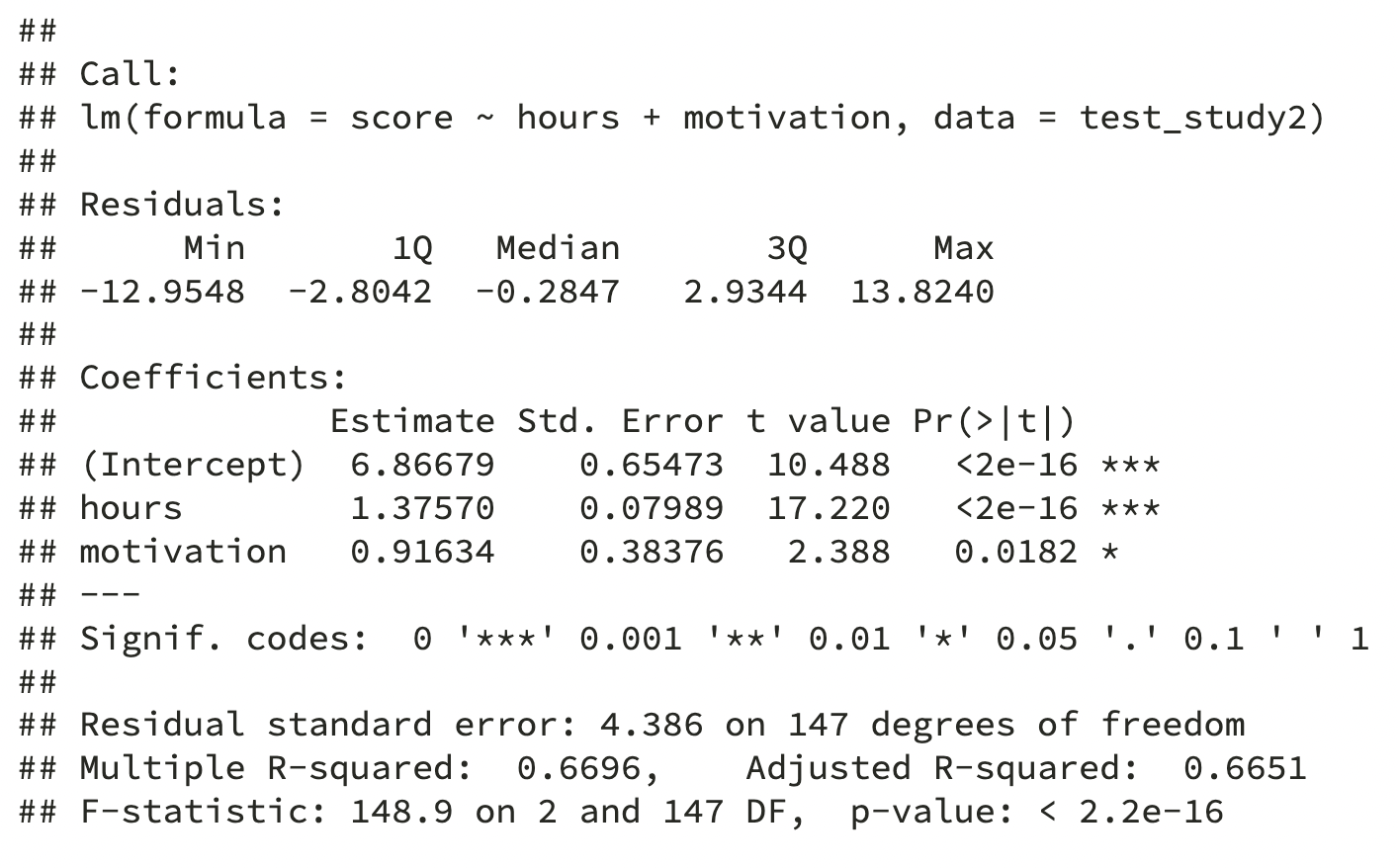

• Based on adjusted R-squared, hours studying and student motivation explain 66.5% of the variance in test scores

• As the sample size is large and the number of predictors small, unadjusted (0.67) and adjusted R-squared (0.665) are similar

Summary

• We have an inferential test, based on a \(t\)-distribution, for the significance of \(\beta\)

• We can compute confidence intervals that give us more certainty that we have captured the true value of \(\beta\)

• We are more likely to find a statistically significant effect when residuals are small and we have a large sample

• We can assess the degree to which our model explains variance in the outcome based on \(R^2\)

• When we have multiple predictors, we should use the adjusted \(R^2\) to get a more conservative estimate

This Week

Tasks

Attend your lab and work together on the exercises

Complete the weekly quiz

Support

Help each other on the Piazza forum

Attend office hours (see Learn page for details)