class: center, middle, inverse, title-slide # <b>Interactions 1 </b> ## Data Analysis for Psychology in R 2<br><br> ### dapR2 Team ### Department of Psychology<br>The University of Edinburgh --- # Weeks Learning Objectives 1. Understand the concept of an interaction. 2. Interpret interactions for between quantitative variables. 3. Interpret interactions between a quantitative and a binary variable. 4. Understand the principle of marginality and why this impacts modelling choices with interactions. 5. Visualize and probe interactions. --- # Topics for today + Broad principle of interactions and general definitions + Quantitative (continuous) and binary (0-1) variable. + Plotting interactions + Importance of centering --- # Lecture notation + For the next two lectures, we will work with the following equation and notation: `$$y_i = \beta_0 + \beta_1 x_{i} + \beta_2 z_{i} + \beta_3 xz_{i} + \epsilon_i$$` + `\(y\)` is a continuous outcome + `\(x\)` will always be the continuous predictor + `\(z\)` will be either the continuous or binary predictor + Dependent on the type of interaction we are discussing. + `\(xz\)` is their product or interaction predictor --- # General definition + When the effects of one predictor on the outcome differ across levels of another predictor. + Note interactions are symmetrical. + What does this mean? + We can talk about interaction of X with Z, or Z with X. + These are identical. --- # General definition + Categorical*continuous interaction: + The slope of the regression line between a continuous predictor and the outcome is different across levels of a categorical predictor. -- + Continuous*continuous interaction: + The slope of the regression line between a continuous predictor and the outcome changes as the values of a second continuous predictor change. + May have heard this referred to as moderation. -- + Categorical*categorical interaction: + There is a difference in the differences between groups across levels of a second factor. + We will discuss this in the context of linear models for experimental design --- # Interpretation: Categorical*Continuous `$$y_i = \beta_0 + \beta_1 x_{i} + \beta_2 z_{i} + \beta_3 xz_{i} + \epsilon_i$$` + Where `\(z\)` is a binary predictor + `\(\beta_0\)` = Value of `\(y\)` when `\(x\)` and `\(z\)` are 0 + `\(\beta_1\)` = Effect of `\(x\)` (slope) when `\(z\)` = 0 (reference group) + `\(\beta_2\)` = Difference intercept between `\(z\)` = 0 and `\(z\)` = 1, when `\(x\)` = 0. + `\(\beta_3\)` = Difference in slope across levels of `\(z\)` --- # Example: Categorical*Continuous .pull-left[ + Suppose I am conducting a study on how years of service within an organisation predicts salary in two different departments, accounts and store managers. + y = salary (unit = thousands of pounds) + x = years of service + z = Department (0=Store managers, 1=Accounts) ] .pull-right[ ```r salary %>% slice(1:10) ``` ``` ## # A tibble: 10 x 3 ## service salary dept ## <dbl> <dbl> <dbl> ## 1 6.22 60.5 1 ## 2 2.73 22.9 0 ## 3 4.58 48.9 1 ## 4 5.36 49.9 1 ## 5 3.53 28.2 0 ## 6 5.63 54.1 1 ## 7 5.65 37.8 0 ## 8 2.61 37.9 1 ## 9 5.94 36.5 0 ## 10 4.94 28.4 0 ``` ] --- # Visualize the data .pull-left[ ```r salary %>% ggplot(., aes(x = service, y = salary)) + geom_point() + xlim(0,8) + labs(x = "Years of Service", y = "Salary (£1000)") ``` ] .pull-right[ 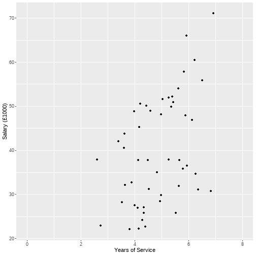<!-- --> ] --- # Visualize the data .pull-left[ ```r salary %>% ggplot(., aes(x = service, y = salary, colour = factor(dept))) + geom_point() + xlim(0,8) + labs(x = "Years of Service", y = "Salary (£1000)") + scale_colour_discrete( name ="Department", breaks=c("1", "0"), labels=c("Accounts", "Store Manager")) ``` ] .pull-right[ 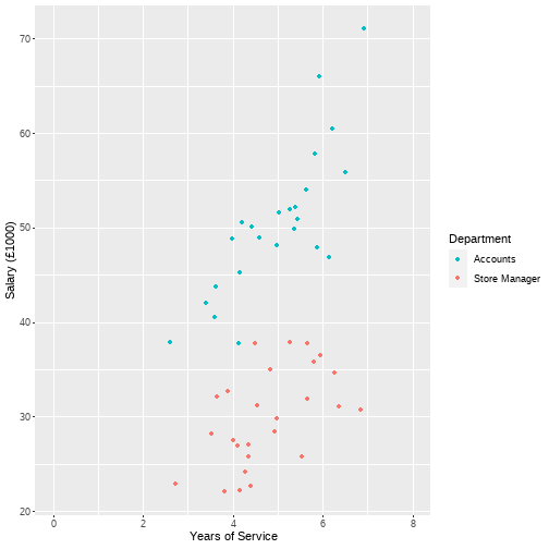<!-- --> ] --- # Example: Full results ```r int <- lm(salary ~ service + dept + service*dept, data = salary) *summary(int) ``` --- # Example: Full results ``` ## ## Call: ## lm(formula = salary ~ service + dept + service * dept, data = salary) ## ## Residuals: ## Min 1Q Median 3Q Max ## -10.3320 -2.7217 -0.2861 2.8132 9.9405 ## ## Coefficients: ## Estimate Std. Error t value Pr(>|t|) ## (Intercept) 16.9023 4.5013 3.755 0.000486 *** ## service 2.7290 0.9227 2.958 0.004882 ** ## dept 4.5395 6.3213 0.718 0.476309 ## service:dept 3.1071 1.2704 2.446 0.018338 * ## --- ## Signif. codes: 0 '***' 0.001 '**' 0.01 '*' 0.05 '.' 0.1 ' ' 1 ## ## Residual standard error: 4.607 on 46 degrees of freedom ## Multiple R-squared: 0.8672, Adjusted R-squared: 0.8585 ## F-statistic: 100.1 on 3 and 46 DF, p-value: < 2.2e-16 ``` --- # Example: Categorical*Continuous + **Intercept** ( `\(\beta_0\)` ): + Predicted salary for a store manager (`dept`=0) with 0 years of service is 16.90. + Noting scale = £16,900 -- + **Service** ( `\(\beta_1\)` ): + For each additional year of service for a store manager (`dept` = 0), salary increases by 2.73. + noting scale = £2,730 -- + **Dept** ( `\(\beta_2\)` ): + Difference in salary between store managers (`dept` = 0) and accounts (`dept` = 1) with 0 years of service is 4.54. + £4,540 -- + **Service:dept** ( `\(\beta_3\)` ): + The difference in slope. For each year of service, those in accounts (`dept` = 1) increase by an additional 3.11. + £3,110 --- # Example: Categorical*Continuous .pull-left[ + **Intercept** ( `\(\beta_0\)` ): Predicted salary for a store manager (`dept`=0) with 0 years of service is 16.90. + **Service** ( `\(\beta_1\)` ): For each additional year of service for a store manager (`dept` = 0), salary increases by 2.73. + **Dept** ( `\(\beta_2\)` ): Difference in salary between store managers (`dept` = 0) and accounts (`dept` = 1) with 0 years of service is 4.54. + **Service:dept** ( `\(\beta_3\)` ): The difference in slope. For each year of service, those in accounts (`dept` = 1) increase by an additional 3.11. ] .pull-right[ <!-- --> ] --- class: center, middle # Time for a break **Quiz time!** Try and answer the following questions to see how you are understanding the plots --- class: center, middle # Welcome Back! **Where we left off... ** We are now going to talk a little about the plots we have been looking at... --- # Plotting interactions .pull-left[ + Simple slopes: + **Regression of the outcome Y on a predictor X at specific values of an interacting variable Z.** + So specifically for our example: + Slopes for salary on years of service at specific values of department. + As department is binary, it takes only two values (0 & 1) + Two simple slopes, one for store managers and one for accounts. ] .pull-right[ <!-- --> ] --- # Simple slopes + When calculating simple slopes, the regression equation is re-ordered to more accurately represent the above definition: `$$\hat{y} = (\beta_1 + \beta_3z)x + (\beta_2z + \beta_0)$$` + `\((\beta_1 + \beta_3z)x\)` captures coefficients for the slope + `\((\beta_2z + \beta_0)\)` captures coefficients for the intercept --- # Example: Categorical*Continuous + So in our example (for `Dept` = 1, accounts): `$$\hat{y} = (\beta_1 + \beta_3z)x + (\beta_2z + \beta_0)$$` `$$\hat{y} = (\beta_1 + \beta_3*1)x + (\beta_2*1 + \beta_0)$$` `$$\hat{salary} = (2.73 + (3.11*1))service + ((4.54*1) + 16.90)$$` `$$\hat{salary} = (5.84)service + (21.34)$$` --- # Example: Categorical*Continuous + So in our example (for `Dept` = 0, store managers): `$$\hat{y} = (\beta_1 + \beta_3z)x + (\beta_2z + \beta_0)$$` `$$\hat{y} = (\beta_1 + \beta_3*0)x + (\beta_2*0 + \beta_0)$$` `$$\hat{salary} = (\beta_1)service + (\beta_0)$$` `$$\hat{salary} = (2.73)service + (16.90)$$` --- # Example: Categorical*Continuous .pull-left[ + Accounts: `$$\hat{salary} = (5.84)service + (21.34)$$` + Store Managers: `$$\hat{salary} = (2.73)service + (16.90)$$` ] .pull-right[ <!-- --> ] --- class: center, middle # Time for a break **No specific task** Just take a few minutes to think about the previous slides. Interactions can be tricky. Add any questions to the discussion board. --- class: center, middle # Welcome Back! **Where we left off... ** So have estimated and visualized interactions Now lets look at a few details of fitting and interpretation --- # Marginal effects + Recall when we have a linear model with multiple predictors, we interpret the `\(\beta_j\)` as the effect "holding all other variables constant". + Also note, with interactions, the effect of `\(x\)` on `\(y\)` changes dependent on the value of `\(z\)`. + More formally, it is the effect of `\(x\)` is conditional on `\(z\)` and vice versa. + What this means is that we can no longer talk about holding an effect constant. + In the presence of an interaction, by definition, this effect changes. + So where as in a linear model without an interaction `\(\beta_j\)` = main effects, with an interaction we refer to **marginal** or **conditional** main effects. --- # Practical implication for modelling `$$y_i = \beta_0 + \beta_1 x_{i} + \beta_2 z_{i} + \beta_3 xz_{i} + \epsilon_i$$` + When we include a higher-order term/interaction in our models ( `\(\beta_3\)` ), it is critical we include the main effects ( `\(\beta_1\)` , `\(\beta_2\)` ). + Without marginal main effects, the single term represents all effects. + Consider dropping `\(\beta_2\)` in our example (difference in the intercept for groups coded 0 and 1) + Common intercept. + Also, if there is a known interaction, we should always include it, otherwise our estimates of `\(\beta_1\)` and `\(\beta_2\)` will be inaccurate. --- # Specifying Interactions in R + How we specify the interactions in R impacts whether it defaults to giving marginal/conditional main effects. + For interactions we can use `*` or `:` + These provide full model results: ```r lm(salary ~ service + dept +service*dept , data = df ) lm(salary ~ service + dept +service:dept , data = df ) lm(salary ~ service*dept , data = df ) ``` + This does not: ```r lm(salary ~ service:dept , data = df ) ``` --- # Centering predictors **Why centre?** + Meaningful interpretation. + Interpretation of models with interactions involves evaluation when other variables = 0. + This makes it quite important that 0 is meaningful in some way. + Note this is simple with categorical variables. + We code our reference group as 0 in all dummy variables. + For continuous variables, we need a meaningful 0 point. --- # Example of age + Suppose I have age as a variable in my study with a range of 30 to 85. + Age = 0 is not that meaningful. + Essentially means all my parameters are evaluated at point of birth. + So what might be meaningful? + Average age? (mean centering) + A fixed point? (e.g. 66 if studying retirement) --- # Centering predictors **Why centre?** + Meaningful interpretation. + Reduce multi-collinearity. + `\(x\)` and `\(z\)` are by definition correlated with the product term `\(XZ\)`. + This produces something call **multi-collinearity** + We will talk more about this next week. + In short, it something we want to avoid. --- # Impact of centering + Remember that our `\(\beta\)` are marginal effects when the other variables = 0 + When we center, we move where 0 is. + So this effects our estimates. --- # Example: Center on minimum value .pull-left[ 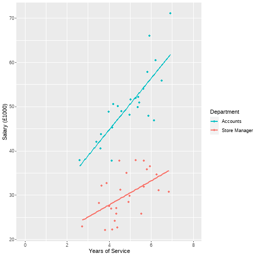<!-- --> ] .pull-right[ 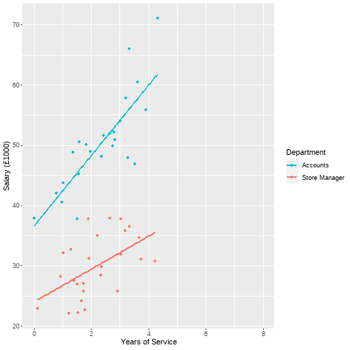<!-- --> ] --- # Example: Mean center .pull-left[ <!-- --> ] .pull-right[ <!-- --> ] --- # Comparing coefficients <table class="table" style="width: auto !important; margin-left: auto; margin-right: auto;"> <thead> <tr> <th style="text-align:left;"> Coefficient </th> <th style="text-align:right;"> Original </th> <th style="text-align:right;"> Minimum </th> <th style="text-align:right;"> Mean </th> </tr> </thead> <tbody> <tr> <td style="text-align:left;"> Intercept </td> <td style="text-align:right;"> 16.90 </td> <td style="text-align:right;"> 24.02 </td> <td style="text-align:right;"> 30.19 </td> </tr> <tr> <td style="text-align:left;"> Service </td> <td style="text-align:right;"> 2.73 </td> <td style="text-align:right;"> 2.73 </td> <td style="text-align:right;"> 2.73 </td> </tr> <tr> <td style="text-align:left;"> Department </td> <td style="text-align:right;"> 4.54 </td> <td style="text-align:right;"> 12.64 </td> <td style="text-align:right;"> 19.67 </td> </tr> <tr> <td style="text-align:left;"> Interaction </td> <td style="text-align:right;"> 3.11 </td> <td style="text-align:right;"> 3.11 </td> <td style="text-align:right;"> 3.11 </td> </tr> </tbody> </table> --- # Summary of today + Interactions tell us whether an effect of a predictor on an outcome changes dependent on the value of a second predictor. + We have considered categorical*continuous interactions today. + Different slopes within groups + And looked at how to visualize and calculate simple slopes --- # Additional Interactions Reading(not compulsory!!) + Aiken, L. S., & West, S. G. (1991). *Multiple regression: Testing and interpreting interactions* . Newbury Park, CA: Sage . + McClelland , G. H., & Judd, C. M. (1993). Statistical difficulties of detecting interactions and moderator effects. *Psychological bulletin* , *114* (2), 376 . + Preacher, K. J. (2015). Advances in mediation analysis: A survey and synthesis of new developments. *Annual Review of Psychology* , *66* , 825-852. --- class: center, middle # Thanks for listening!