LM & One-way Designs

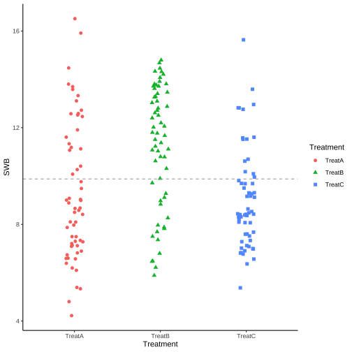
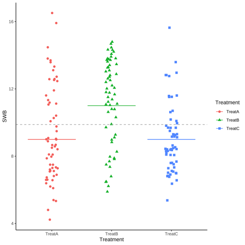
class: center, middle, inverse, title-slide

# <b>LM & One-way Designs </b>
## Data Analysis for Psychology in R 2<br><br>
### Tom Booth & Alex Doumas
### Department of Psychology<br>The University of Edinburgh
### AY 2020-2021

---

# Weeks Learning Objectives
1. Recap on experimental designs and types of data structure.

2. Understand the distinction between simple, main and interaction effects for experimental designs.

3. Understand the distinction between simple, main, and interaction effects.

---
# Topics for today
+ Testing experimental effects in linear models

+ Introduce our example for the next two weeks

+ One-way design example

---
# Hypotheses we test in experimental studies

+ One-way designs:
  + **Main effect (tests overall effect of a condition; `$F$`-tests )**
  + Contrasts (tests differences between specific group means; `$\beta$` )

+ Factorial designs:
  + Simple contrasts/effects
  + Interactions (categorical*categorical)
  + Main effects

---
# Example
+ The data comes from a study into patient care in a paediatric wards.

+ A researcher was interested in whether the subjective well-being of patients differed dependent on the post-operation treatment schedule they were given, and the hospital in which they were staying.

+ **Condition 1**: `Treatment` (Levels: TreatA, TreatB, TreatC).
  
+ **Condition 2**: `Hosp` (Levels: Hosp1, Hosp2). 
  
+ Total sample n = 180 (30 patients in each of 6 groups).
  + Between person design.

+ **Outcome**: Subjective well-being (SWB)
  + An average of multiple raters (the patient, a member of their family, and a friend). 
  + SWB score ranged from 0 to 20.

---
# The data

```r
hosp_tbl <- read_csv("hospital.csv", col_types = "dff")
hosp_tbl %>%
  slice(1:10)
```

```
## # A tibble: 10 x 3
##      SWB Treatment Hospital
##    <dbl> <fct>     <fct>   
##  1   6.2 TreatA    Hosp1   
##  2  15.9 TreatA    Hosp1   
##  3   7.2 TreatA    Hosp1   
##  4  11.3 TreatA    Hosp1   
##  5  11.2 TreatA    Hosp1   
##  6   9   TreatA    Hosp1   
##  7  14.5 TreatA    Hosp1   
##  8   7.3 TreatA    Hosp1   
##  9  13.7 TreatA    Hosp1   
## 10  12.6 TreatA    Hosp1
```

---
# For today

+ As we are discussing one-way designs, today we will just look at the effect of treatment on SWB.

+ What we will show is that:

```r
lm(SWB ~ Treatment, data = hosp_tbl)
```

+ and

```r
aov(SWB ~ Treatment, data = hosp_tbl)
```

+ are the same.

---
# Descriptive statistics by group

```r
hosp_tbl %>%
  select(1:2) %>%
  group_by(Treatment) %>%
  summarise(
    mean = round(mean(SWB)),
    sd = round(sd(SWB),1),
    N = n()
  )
```

```
## `summarise()` ungrouping output (override with `.groups` argument)
```

```
## # A tibble: 3 x 4
##   Treatment  mean    sd     N
##   <fct>     <dbl> <dbl> <int>
## 1 TreatA        9   2.9    60
## 2 TreatB       11   2.5    60
## 3 TreatC        9   2      60
```

---
# Sums of squares for ANOVA and LM
+ Recall that in ANOVA we break down sums of squares

`$$SS_{total} = SS_{between} + SS_{within}$$`

+ And that `$SS_{between}$` refers to the conditions/groups.
  + This group structure is the model.

+ Hence we have a direct parallel to linear model

`$$SS_{total} = SS_{model} + SS_{residual}$$`

---
# Total Variation & SS

.pull-left[

![](dapR2_lec22_Oneway_files/figure-html/unnamed-chunk-6-1.png)

]

.pull-right[

`$$SS_{total} = \sum(Y_{ij} - \bar{Y})^2$$`

+ The subscript `$ij$` here denotes individuals within groups.

+ Other than this, this is identical to the linear model.

+ It is the sum of the square deviations around the mean (dashed grey line)

]

---
# Between/Model variation & SS

.pull-left[

![](dapR2_lec22_Oneway_files/figure-html/unnamed-chunk-7-1.png)

]

.pull-right[

`$$SS_{between} = \sum n(\bar{Y_j} - \bar{Y})^2$$`

+ Sum of the squared deviations of the group means from the mean of Y.
  + The solid coloured lines to the dashed grey line

+ For linear model, we stated

`$$SS_{Model} = \sum_{i=1}^{n}(\hat{y}_i - \bar{y})^2$$`

+ These are equivalent. Remember
  + `$\hat{y_i}$` = model predicted value
  + So this is equal to the deviation of the the model predicted value of `$y$` for a given value of `$x$`
  + When we have categorical predictors, the predicted value of `$y$` for a given value of `$x$` = group mean

]

---
# Within/residual variation & SS

.pull-left[

![](dapR2_lec22_Oneway_files/figure-html/unnamed-chunk-8-1.png)

]

.pull-right[

`$$SS_{within} = \sum(Y_{ij} - \bar{Y_j})^2$$`
+ Sum of the squared deviations of the individual values from the group mean.

+ For the linear model we stated

`$$SS_{Residual} = \sum_{i=1}^{n}(y_i - \hat{y}_i)^2$$`
+ And as in the previous slide, these are equivalent because predicted value for a given value of `$x$` is the group mean.

+ Or put another way, our model = group means.

]

---
# F-test in LM and ANOVA

**ANOVA**
<table class="table" style="width: auto !important; margin-left: auto; margin-right: auto;">
 <thead>
  <tr>
   <th style="text-align:left;"> SS </th>
   <th style="text-align:left;"> df </th>
   <th style="text-align:left;"> MS </th>
   <th style="text-align:left;"> Fratio </th>
   <th style="text-align:left;"> pvalue </th>
  </tr>
 </thead>
<tbody>
  <tr>
   <td style="text-align:left;"> Between </td>
   <td style="text-align:left;"> g-1 </td>
   <td style="text-align:left;"> SS between/df between </td>
   <td style="text-align:left;"> MS between/ MS within </td>
   <td style="text-align:left;"> F(df between,df within) </td>
  </tr>
  <tr>
   <td style="text-align:left;"> Within </td>
   <td style="text-align:left;"> g(n-1) </td>
   <td style="text-align:left;"> SS within/df within </td>
   <td style="text-align:left;">  </td>
   <td style="text-align:left;">  </td>
  </tr>
  <tr>
   <td style="text-align:left;"> Total </td>
   <td style="text-align:left;"> gn-1 </td>
   <td style="text-align:left;">  </td>
   <td style="text-align:left;">  </td>
   <td style="text-align:left;">  </td>
  </tr>
</tbody>
</table>

+ g = number of levels or groups in condition (g=3)
+ n = number of participants per group (n=60)

+ So here:
  + `$df_{between}$` = 3-1 = 2
  + `$df_{within}$` = 3*(60-1) = 177
  + `$df_{total}$` = (3*60)-1 = 179

---
# F-test in LM and ANOVA

**Linear Model**

<table class="table" style="width: auto !important; margin-left: auto; margin-right: auto;">
 <thead>
  <tr>
   <th style="text-align:left;"> SS </th>
   <th style="text-align:left;"> df </th>
   <th style="text-align:left;"> MS </th>
   <th style="text-align:left;"> Fratio </th>
   <th style="text-align:left;"> pvalue </th>
  </tr>
 </thead>
<tbody>
  <tr>
   <td style="text-align:left;"> Model </td>
   <td style="text-align:left;"> k </td>
   <td style="text-align:left;"> SS model/df model </td>
   <td style="text-align:left;"> MS model/ MS residual </td>
   <td style="text-align:left;"> F(df model,df residual) </td>
  </tr>
  <tr>
   <td style="text-align:left;"> Residual </td>
   <td style="text-align:left;"> n-k-1 </td>
   <td style="text-align:left;"> SS residual/df residual </td>
   <td style="text-align:left;">  </td>
   <td style="text-align:left;">  </td>
  </tr>
  <tr>
   <td style="text-align:left;"> Total </td>
   <td style="text-align:left;"> n-1 </td>
   <td style="text-align:left;">  </td>
   <td style="text-align:left;">  </td>
   <td style="text-align:left;">  </td>
  </tr>
</tbody>
</table>

+ k = number of predictors
+ n = sample size

+ So here:
  + `$df_{model}$` = k = 2
  + `$df_{residual}$` = 180-2-1 = 177
  + `$df_{total}$` = 180-1 = 179

---
# In R

```r
summary(aov(SWB ~ Treatment, data = hosp_tbl))
```

```
##              Df Sum Sq Mean Sq F value  Pr(>F)    
## Treatment     2    177   88.51   14.04 2.2e-06 ***
## Residuals   177   1116    6.31                    
## ---
## Signif. codes:  0 '***' 0.001 '**' 0.01 '*' 0.05 '.' 0.1 ' ' 1
```

---
# In R

```r
summary(lm(SWB ~ Treatment, data = hosp_tbl))
```

```
## 
## Call:
## lm(formula = SWB ~ Treatment, data = hosp_tbl)
## 
## Residuals:
##    Min     1Q Median     3Q    Max 
## -5.373 -1.987 -0.300  1.838  7.173 
## 
## Coefficients:
##                 Estimate Std. Error t value Pr(>|t|)    
## (Intercept)       9.3267     0.3242  28.770  < 2e-16 ***
## TreatmentTreatB   1.9467     0.4585   4.246 3.51e-05 ***
## TreatmentTreatC  -0.2850     0.4585  -0.622    0.535    
## ---
## Signif. codes:  0 '***' 0.001 '**' 0.01 '*' 0.05 '.' 0.1 ' ' 1
## 
## Residual standard error: 2.511 on 177 degrees of freedom
## Multiple R-squared:  0.1369,	Adjusted R-squared:  0.1271 
## F-statistic: 14.04 on 2 and 177 DF,  p-value: 2.196e-06
```

---
# Summary of today

+ We introduced our example, and focussed on the effect of the treatments

+ And looked at the calculation of `$F$`-test

+ Key point:
  + It is exactly the same test.
  + Always keep in mind that the group structure = model

---
# Next tasks
+ This week:
  + Complete your lab
  + Come to office hours
  + Weekly quiz - content from week 10
      + Open Monday 09:00
      + Closes Sunday 17:00