Week 5: LM Case Diagnostics

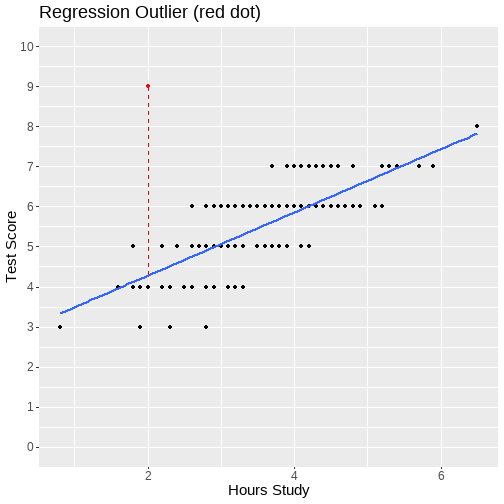
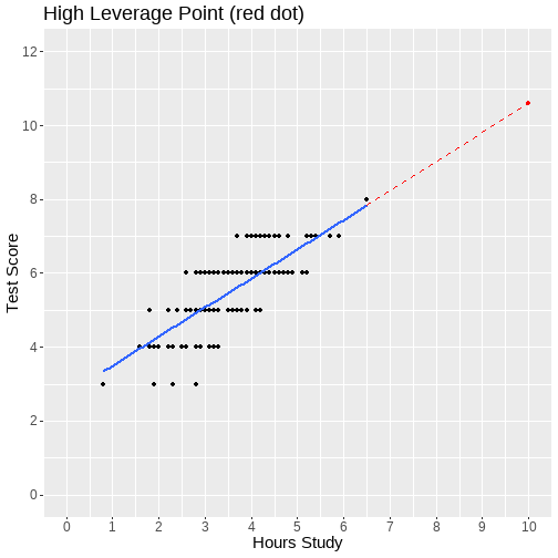
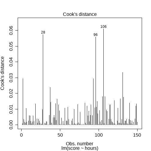
class: center, middle, inverse, title-slide

# <b>Week 5: LM Case Diagnostics </b>
## Data Analysis for Psychology in R 2<br><br>
### TOM BOOTH & ALEX DOUMAS
### Department of Psychology<br>The University of Edinburgh
### AY 2020-2021

---

# Week's Learning Objectives

1. Understand the difference between outliers and influential points.

2. Understand and apply methods to detect outliers and influential points.

3. Comment on the issues of correlation vs causation and generalisability of the sample results.

4. Run a full simple linear model analysis from start to finish and to correctly interpret the results.

---
# Topics for today

+ Linear model outliers

+ Leverage

+ Influence

+ Dealing with problematic cases

---
#  Linear model diagnostics

+ In previous lectures we have discussed evaluating linear models:
	+ Evaluating model fit ( `$R^2$` and `$F$`-ratio )
	+ Evaluating individual predictors
	+ Evaluating assumptions

+ Another important aspect of evaluating linear models pertains to the cases (individuals):
	+ Does the model fit poorly for some individuals?
	+ Do some individuals have a lot of influence on the results?

+ Linear model diagnostics allow us to explore individual cases in the context of a model

---
#  Three important features

+ Model outliers
	+ Cases for which there is a large discrepancy between their predicted value ( `$\hat{y_i}$` ) and their observed value ( `$y_i$` )

+ High leverage cases
	+ Cases with an unusual value of the predictor ( `$x_i$` )

+ High influence cases
	+ Cases who are having a large impact on the estimation of model

---
#  Model outliers

+ Linear model outliers are cases that have unusual outcome values given their predictor values
	+ They will show a large difference between the predicted ( `$\hat{y_i}$` ) and the observed value ( `$y_i$` )

+ **What quantity have we calculated that would summarise this difference?**

+ Outliers will demonstrate large **residuals** ( `$\epsilon_i$` )
  + If you got stuck here, look back at the introduction to linear models

---
#  Why are we interested in linear model outliers?

.pull-left[
+ They can (but do not necessarily) have a strong influence on the model
	+ We'll get to this.

+ It may be informative to follow-up and investigate outliers
	+ Is it a data entry error?
	+ Does the case somehow not belong with the rest of the data? (E.g., a male in a sample of females)
]

.pull-right[
![](dapR2_lec09_LMdiagnostics_files/figure-html/unnamed-chunk-2-1.png)

]

---
#  How do we determine if a case is an outlier?

+ We judge linear model outlying-ness of a case on the basis of the size of its residual

+ Unstandardised residuals are:

`$$y_i - \hat{y_i}$$`

+ They are in the same units as the DV

+ Fine for comparison across cases within the same linear model model

+ Difficult to compare across models where the DVs will have different units

---
#  Standardised residuals

+ **Standardised residuals**
	+ Divide the unstandardised residuals by an estimate of their standard deviation
	+ Converts the residuals to z-score units
	+ However, their calculation includes the potential outlier

+ **Studentised residuals**
	+ Provide a version of the standardised residual excluding the case
	+ Values **>+2 or <-2** indicate potential outlyingness

---
#  Identifying studentised residuals >2

.pull-left[

```r
m1 <- lm(score ~ hours, data = df)

df %>%
  mutate(
*   resid = rstudent(m1)
  ) %>%
* filter(., resid > 2 | resid < -2) %>%
  kable(.)  %>%
  kable_styling(., full_width = F)
```
]

.pull-right[

+ Steps:
  + Extract the studentized residuals from our model.
  + Identify those outside `$\pm > 2$`
]

---
#  Identifying studentised residuals >2

.pull-left[

```r
m1 <- lm(score ~ hours, data = df)

df %>%
  mutate(
*   resid = rstudent(m1)
  ) %>%
* filter(., resid > 2 | resid < -2) %>%
  kable(.)  %>%
  kable_styling(., full_width = F)
```
]

.pull-right[

---
#  Leverage 
.pull-left[
+ High leverage cases are those with an unusual predictor value or combination of predictor values
	+ In simple linear model: an `$x$` value far from the `$\bar{x}$`

+ **Why are we interested in leverage?** 
+ High leverage cases have potential to influence `$\hat \beta_0$` and `$\hat \beta_1$` 
]

.pull-right[
![](dapR2_lec09_LMdiagnostics_files/figure-html/unnamed-chunk-6-1.png)
]

---
#  Finding a case with high leverage

+ **Hat values** ( `$h_i$` ) are used to assess leverage in linear model

+ For a simple linear model, the hat value for case `$i$` would be:

`$$h_i = \frac{1}{n} + \frac{(x_i - \bar{x})^2}{\sum_{i=1}^n(x_i - \bar{x})^2}$$`

+ Where:
  + `$n$` is the sample size
  + `$(x_i - \bar{x})^2$` is the squared deviation of the predictor value for that case, `$x_i$`, from the mean `$\bar x$`
  + `$\sum_i^n(x_i - \bar{x})^2$` is the sum of all these squared deviations, for all cases

---
#  Finding a case with high leverage

+ The mean of hat values ( `$\bar{h}$` ) is then:

`$$\bar{h} = (k+1)/n$$`

+ `$k$` is the number of predictors
  + `$n$` is the sample size

+ In simple linear regression `$k = 1$` as there is just one predictor, hence `$\bar h = (1 + 1) / n = 2 /n$`

+ As a rough heuristic, values more than `$2\bar{h}$` are considered high leverage

---
#  Hat values in R

.pull-left[

```r
df %>%
  mutate(
*   hat = hatvalues(m1)
  ) %>%
* filter(., hat > 2*((1+1)/150)) %>%
  kable(.)  %>%
  kable_styling(., full_width = F)
```

]

.pull-right[

+ Steps to identify large `$h_i$` values:
  + Extract the `$h_i$` from our model.
  + Identify those outside `$2\bar{h}$`
  
]

---
#  Hat values in R

.pull-left[

```r
df %>%
  mutate(
*   hat = hatvalues(m1)
  ) %>%
* filter(., hat > 2*((1+1)/150)) %>%
  kable(.)  %>%
  kable_styling(., full_width = F)
```

]

.pull-right[

<table class="table" style="width: auto !important; margin-left: auto; margin-right: auto;">
 <thead>
  <tr>
   <th style="text-align:left;"> ID </th>
   <th style="text-align:right;"> score </th>
   <th style="text-align:right;"> hours </th>
   <th style="text-align:right;"> study </th>
   <th style="text-align:right;"> hat </th>
  </tr>
 </thead>
<tbody>
  <tr>
   <td style="text-align:left;"> ID12 </td>
   <td style="text-align:right;"> 7 </td>
   <td style="text-align:right;"> 5.7 </td>
   <td style="text-align:right;"> 1 </td>
   <td style="text-align:right;"> 0.0413732 </td>
  </tr>
  <tr>
   <td style="text-align:left;"> ID26 </td>
   <td style="text-align:right;"> 4 </td>
   <td style="text-align:right;"> 1.8 </td>
   <td style="text-align:right;"> 0 </td>
   <td style="text-align:right;"> 0.0318169 </td>
  </tr>
  <tr>
   <td style="text-align:left;"> ID28 </td>
   <td style="text-align:right;"> 3 </td>
   <td style="text-align:right;"> 1.9 </td>
   <td style="text-align:right;"> 0 </td>
   <td style="text-align:right;"> 0.0290902 </td>
  </tr>
  <tr>
   <td style="text-align:left;"> ID37 </td>
   <td style="text-align:right;"> 6 </td>
   <td style="text-align:right;"> 5.2 </td>
   <td style="text-align:right;"> 1 </td>
   <td style="text-align:right;"> 0.0268537 </td>
  </tr>
  <tr>
   <td style="text-align:left;"> ID49 </td>
   <td style="text-align:right;"> 7 </td>
   <td style="text-align:right;"> 5.9 </td>
   <td style="text-align:right;"> 0 </td>
   <td style="text-align:right;"> 0.0482759 </td>
  </tr>
  <tr>
   <td style="text-align:left;"> ID54 </td>
   <td style="text-align:right;"> 7 </td>
   <td style="text-align:right;"> 5.7 </td>
   <td style="text-align:right;"> 1 </td>
   <td style="text-align:right;"> 0.0413732 </td>
  </tr>
  <tr>
   <td style="text-align:left;"> ID57 </td>
   <td style="text-align:right;"> 4 </td>
   <td style="text-align:right;"> 1.6 </td>
   <td style="text-align:right;"> 0 </td>
   <td style="text-align:right;"> 0.0377394 </td>
  </tr>
  <tr>
   <td style="text-align:left;"> ID60 </td>
   <td style="text-align:right;"> 3 </td>
   <td style="text-align:right;"> 0.8 </td>
   <td style="text-align:right;"> 0 </td>
   <td style="text-align:right;"> 0.0676857 </td>
  </tr>
  <tr>
   <td style="text-align:left;"> ID71 </td>
   <td style="text-align:right;"> 7 </td>
   <td style="text-align:right;"> 5.4 </td>
   <td style="text-align:right;"> 1 </td>
   <td style="text-align:right;"> 0.0321923 </td>
  </tr>
  <tr>
   <td style="text-align:left;"> ID74 </td>
   <td style="text-align:right;"> 7 </td>
   <td style="text-align:right;"> 5.2 </td>
   <td style="text-align:right;"> 1 </td>
   <td style="text-align:right;"> 0.0268537 </td>
  </tr>
  <tr>
   <td style="text-align:left;"> ID80 </td>
   <td style="text-align:right;"> 7 </td>
   <td style="text-align:right;"> 5.3 </td>
   <td style="text-align:right;"> 1 </td>
   <td style="text-align:right;"> 0.0294448 </td>
  </tr>
  <tr>
   <td style="text-align:left;"> ID118 </td>
   <td style="text-align:right;"> 4 </td>
   <td style="text-align:right;"> 1.9 </td>
   <td style="text-align:right;"> 0 </td>
   <td style="text-align:right;"> 0.0290902 </td>
  </tr>
  <tr>
   <td style="text-align:left;"> ID131 </td>
   <td style="text-align:right;"> 5 </td>
   <td style="text-align:right;"> 1.8 </td>
   <td style="text-align:right;"> 0 </td>
   <td style="text-align:right;"> 0.0318169 </td>
  </tr>
  <tr>
   <td style="text-align:left;"> ID141 </td>
   <td style="text-align:right;"> 8 </td>
   <td style="text-align:right;"> 6.5 </td>
   <td style="text-align:right;"> 1 </td>
   <td style="text-align:right;"> 0.0727376 </td>
  </tr>
</tbody>
</table>
  
]

---
class: center, middle
# Time for a break

Let's have a R task.

Look at the code of the previous slide

Write in words what each line is doing

Answer will be posted in the week 5 folder.

---
class: center, middle
# Welcome Back!

**Where we left off... **

We had discussed outliers and leverage.

Next up, influence.

---
#  Influence

+ High leverage cases, when they are also linear model outliers, will have high **influence**

+ Cases with high influence, have a strong effect on the coefficients

+ If we deleted such a case, the linear model coefficients would change substantially

---
# Influence

+ If a handful of influential cases are responsible for the linear model results, the conclusions might not generalise very well

+ Multiple ways to consider influence.
  + Here we will discuss Cook's distance.
  + In a few weeks we will consider some additional measures
  
+ Cook's Distance of a data point `$i$` (can be written many ways):

`$$D_i = \frac{(\text{StandardizedResidual}_i)^2}{k+1} \times \frac{h_i}{1-h_i}$$`

---
#  Cooks Distance 
`$$\frac{(\text{StandardizedResidual}_i)^2}{k+1} = \text{Outlyingness}$$`

`$$\frac{h_i}{1-h_i} = \text{Leverage}$$`

+ So `$D_i = \text{Outlyingness} \times \text{Leverage}$`

+ Cook's distance refers to **the average distance the `$\hat{y}$` values will move if a given case is removed.**
  + If removing one case changes the predicted values a lot (moves the regression line), then that case is influencing our results.

---
#  Cooks Distance

+ Many different suggestions for cut-off's:
  + `$D_i > 1$` 
  + `$D_i > \frac{4}{n-k-1}$`
  + Or size relative all values in data set

---
#  Cook's distance in R

.pull-left[

```r
df %>%
  mutate(
*   cook = cooks.distance(m1)
  ) %>%
* filter(., cook > 4/(150-1-1)) %>%
  kable(.)  %>%
  kable_styling(., full_width = F)
```

]

.pull-right[
![](dapR2_lec09_LMdiagnostics_files/figure-html/unnamed-chunk-11-1.png)

]

---
#  What should be done about outliers, high leverage and high influence values?

+ Easier to identify unusual cases than it is to decide what to do about them?

+ In general, not a good idea to delete cases automatically for exceeding a threshold. 
	+ Especially if they don't show large influence
	
+ Instead, try to investigate why a case is unusual

+ Think of linear model diagnostics more as a way of learning about the limitations of the model
	+ Which cases can't it explain very well?
	+ Why is that?
	+ Do results depend quite strongly on certain cases?

---
#  Investigating and dealing with unusual cases

+ Is there a data entry error?
	+ Is the value within the plausible range of values for a variable?
	+ Can it be corrected? If not, the incorrect value should be deleted

+ Is the data legitimate but extreme?
	+ Consider ways to reduce its influence rather than delete (e.g. **windsorizing**)
	+ May be model specification problems (e.g. missing variables, interactions - coming soon)

+ Are there unusual values as a result of skewness?

???
+ Replacing the extreme value with the next largest value for that variable
+ Avoids missingness/ preserves information
+ Note that deleting or winsorising values can change the model, therefore, different cases might then show up as outlying, high leverage, or influential
+ Iterative approach to removing/ winsorising cases is needed

---
#  Sensitivity Analyses

+ Sensitivity analysis refers to the idea of checking whether you get similar results irrespective of the methodological decisions you make

+ Sensitivity analysis can be used to check whether you get the same pattern of results. Do the estimated regression coefficients change substantially:
	+ With versus without including certain unusual cases?
	+ With versus without transforming a variable?

+ If results are highly similar, you have more confidence that the results aren't very dependent on those decisions

+ If they differ a lot, this should be reported as a limitation
  
---
# Summary

+ We have looked at case diagnostics for lm

+ Outliers can be assessed via studentized residuals.

+ Leverage can be assessed via hat values

+ Influence can be assessed via Cook's distance

+ In short, we do not want a small number of observations having undue influence over our results, so we should always look closely at diagnostics.

---
# Next tasks

+ This week:
  + Complete your lab
  + Come to office hours
  + Weekly quiz: Assessed quiz - Week 4 content.
      + Open Monday 09:00
      + Closes Sunday 17:00