class: center, middle, inverse, title-slide # <b>Week 10: Continuous Probability Distributions </b> ## Data Analysis for Psychology in R 1<br><br> ### ALEX DOUMAS & TOM BOOTH ### Department of Psychology<br>The University of Edinburgh --- # Week's Learning Objectives 1. Understand the key difference between discrete and continuous probability distributions. 2. Review the difference between a PDF and CDF. 3. Apply understanding of continuous probability distributions to the example of a normal distribution. 4. Using a range from a continuous probability distribution. 5. Introduce other continuous probability distributions. --- ## Today - Discrete and continuous probability distributions. - Properties of the normal distribution. - Using ranges from the normal distribution to calculate probability estimates. - The standard normal distribution. - The standard normal distribution and the t distribution. --- ## Discrete vs. continuous - Recall that a discrete probability ditribution describes a random variable that produces a discrete set of outcomes. -- - By contrast, a continuous probability distribution describes a random variable that produces a continuous set of outcomes. -- - As a result, while a discrete probability distribution is jagged, a continuous probability distribution is smooth. -- - What are some examples of contiuous random variables? - Height, RTs, temperature, distance that a ball can be thrown... - If you have arbitrary precision of measurement, you have a continuous random variable. -- - Now, let's take a look at perhaps the most widely used continuous probability distribution... --- ## Normal distribution - This term normal distribution has come up a lot. -- - A normal distribution is a continuous distribution. -- - It is uni-modal (one peak) and symmetrical. -- - Also referred to as the Gaussian distribution. --- ## Normal: PDF $$ f(x|\mu, \sigma) = \frac{1}{\sigma\sqrt{2\pi}}e^{-\frac{(x - \mu)^2}{2\sigma^2}} $$ - A little bit scary! - But the basic points are: - It is a function of data *x* - And *two* parameters `\(\mu\)` and `\(\sigma\)` (mean and SD) --- ## Normal family - There is not one single normal distribution. - We have a family of different distributions defined by the mean, `\(\mu\)`, and standard deviation, `\(\sigma\)`. --- ## Different normals 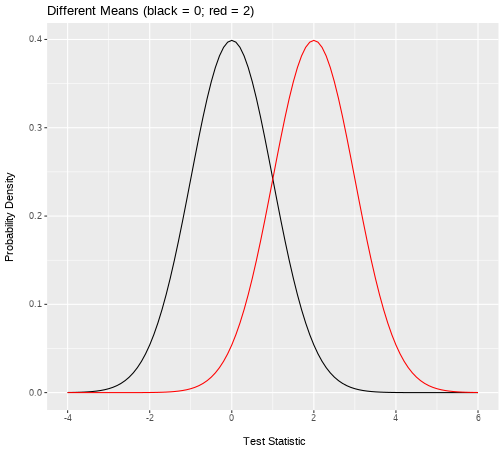<!-- --> --- ## Different normals 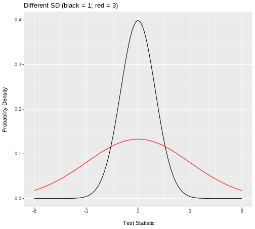<!-- --> --- ## Properties of normal - Nice properties of any normal distribution: - `\(\approx\frac{1}{2}\)` of area falls under `\(\frac{2}{3}\)` of a SD on either side of mean - `\(\approx\frac{2}{3}\)` of area falls under 1 SD on either side of mean. - `\(\approx\)` 95% of area falls under 2 SD on either side of mean. - **Exactly** 95% falls under +/- 1.96 SD - `\(\approx 99.75%\)` of area falls under 3 SD on either side of mean. --- ## Using the PDF of the normal distribution - Let's use the normal disribution to illustrate how continuous probability distributions work. -- - With a discrete random variable it makes sense to ask: 'what's the probability associated with a specific value of the random variable'. - e.g., what the probability of getting heads on a fair coin? -- - With a continuous random variable it makes sense to ask about ranges of scores - e.g., what's the probability of sampling someone between 1.6 and 1.7 meters tall if we sample students from a university? --- ## Using the PDF of the normal distribution .pull-left[ - Let's assume that in some school, height is normally distributed, the mean height is 150 cm and the sd is 20 cm. - We can ask what is the probability of sampling someone between 160cm and 170cm? - This question translates to: `\(p(160 \leq x \leq 170) = ?\)` - Let's unpack asking this question... ] .pull-right[ <!-- --> ] --- ## Using the PDF of the normal distribution .pull-left[ - We are asking: `\(p(160 \leq x \leq 170) = ?\)` - Let's draw these boundries on our plot... ] .pull-right[ 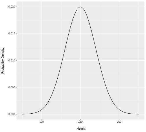<!-- --> ] --- ## Using the PDF of the normal distribution .pull-left[ - `\(p(160 \leq x \leq 170) = ?\)` - What is the value of the area under the curve between these two lines? ] .pull-right[ 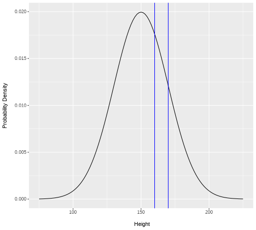<!-- --> ] --- ## Using the PDF of the normal distribution .pull-left[ - We get the area under a curve by calculating an integral `$$\int_{a}^{b} f(a) \,dx$$` - (Don't worry, you do not need to know the details of integrals, but you may encounter the equation above.) - This equation can be read as: The integral of values falling between vertical lines a and b on the function a of variable x - We can calculate this value using the probability density function... ] .pull-right[ <!-- --> ] --- ## Using the PDF of the normal distribution .pull-left[ - *pnorm(x, mean=m, sd=n)* - *x* is an vector; *mean* and *sd* give the parameters of the function - returns the area under the normal distribution (with a mean of m and a sd of n) below x. ```r pnorm(170, mean=150, sd=20) ``` ``` ## [1] 0.8413447 ``` - Now you know the propotion under the curve below 170, so how do we find the area between 160 and 170? - If you subtract from that value the proporiton under the curve below 160, you're left with the proportion under the curve between 160 and 170... ] .pull-right[ <!-- --> ] --- ## Using the PDF of the normal distribution .pull-left[ ```r pnorm(170, mean=150, sd=20) - pnorm(160, mean=150, sd=20) ``` ``` ## [1] 0.1498823 ``` - So we know there is a probability of .15 that someone sampled from this university will have a height between 160 and 170. ] .pull-right[ <!-- --> ] --- ## Using the PDF of the normal distribution .pull-left[ - We can also ask about the probability of a sampled element having a value from one of 2+ ranges. - For example: What is the probability that a person will have a height below 100 or greater than 200? `\(p(x \leq 100 \:or\: x \geq 200)\)` ```r pnorm(100, mean=150, sd=20) ``` ``` ## [1] 0.006209665 ``` ```r 1 - pnorm(200, mean=150, sd=20) ``` ``` ## [1] 0.006209665 ``` - (Why are we subtracting a value from 1 here?) - `\(p(x \leq 100 \:or\: x \geq 200) = p(x \leq 100) + p(x \geq 200) = .006 + .006 = .012\)` ] .pull-right[ <!-- --> ] --- ## Using the PDF of the normal distribution - As a final point, what if I wanted to know where the 5% of the most extreme values (i.e., smallest and largest) in this distribution fall? - First, this distribution is symmetric, which means that there are the same number of extreme values at the bottom and top end. - Second, as the distribution is symmetric the most extreme 5% will be the 2.5% at the bottom of the disribution and the 2.5% at the top. - So, what I want to know is: What is the height below which there are only 2.5% of students, and what is the height above which there are only 2.5% of students? --- ## Using the PDF of the normal distribution .pull-left[ - To find the the value of a probability distribution at which the pdf is x, I use *qnorm(x, mean=m, sd=n)* - So, to get the value below which 2.5% of values occur (for a normal with a mean of 150 and a sd of 20): ```r qnorm(.025, mean=150, sd=20) ``` ``` ## [1] 110.8007 ``` - To to get the value above which 2.5% of values occur (for a normal with a mean of 150 and a sd of 20): ```r qnorm(.975, mean=150, sd=20) ``` ``` ## [1] 189.1993 ``` ] .pull-right[ <!-- --> ] --- ## Remember z-scores $$ Z = \frac{x - \mu}{\sigma} $$ - It is quite typical to present a normal distribution in terms of z-scores. - z-scores standardize values of x. - The numerator: converts x to deviations from the mean. - The denominator: scales these values based on the observed spread in the data (SD) - The result is the standard normal distribution... --- ## Standard normal - The distribution of z-scores is called the standard normal distribution. - It has: - Mean = 0 (why?) - SD = 1 (why?) --- ## An (important) aside: probability and liklihood - In normal english, probability and liklihood mean the same thing. - However, in statistics they (very confusingly) mean similar, but not identical things. - In statistics, if you have a conditional event `\(A|B\)`, then `\(p(A|B) = L(B|A)\)` - Often times we will use probability to refer to possible results (i.e., what is the probability of this kind of world giving us these results-*see above); we will use liklihood to refer to the probability of the world being some way given that we observed some results (e.g., as we do when we have results and want to use that to make an inference about the world). - NOTE: This point isn't that important right now, but it will come up again when we talk about hypothesis testing. --- ## Standard normal vs. t distribution .pull-left[ - The t distribution (it'll come up next semester) is like z scores but replace `\(\sigma\)` with *sd*. - As a result, the tails a bit higher to account for extra variablility (or uncertainty from using estimate rather than actual value). ] .pull-right[ 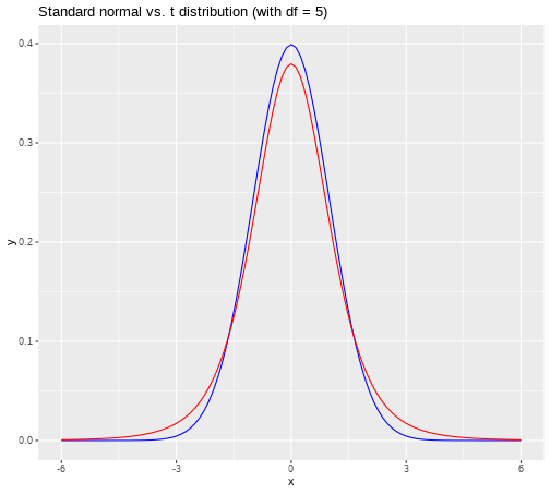<!-- --> ] --- # Summary of today - Continuous probability distributions. - The normal distribution. - Using the normal distribution to make estimates about the probability of events. - The normal distribution and the t-distribution. --- # Next tasks + Next week, we will cover sampling. + This week: + Complete your lab + Come to office hours + Come to Q&A session + Weekly quiz - on week 9 (lect 8) content + Open Monday 09:00 + Closes Sunday 17:00