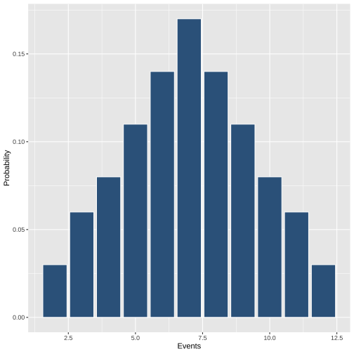
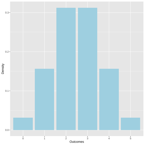
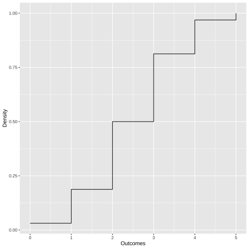
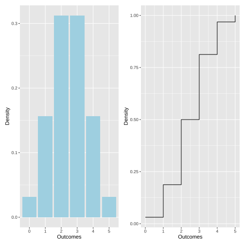
Lecture 8: Discrete Probability Distributions

class: center, middle, inverse, title-slide

# <b>Lecture 8: Discrete Probability Distributions </b>
## Data Analysis for Psychology in R 1<br><br>
### ALEX DOUMAS & TOM BOOTH
### Department of Psychology<br>The University of Edinburgh
### AY 2020-2021

---

# Weeks Learning Objectives
1. Understand concept of a random variable.
2. Understand the process of assigning probabilities to all outcomes.
3. Understand the difference between a probability mass function (PMF) and a cummulative probability function (CDF).
4. Apply the understanding of discrete probability distributions to the example of the binomial distribution.

---
## Today
- What are random variables? 
- Assigning probabilities to outcomes 
- What is a probability distribution? 
- What are probability mass functions and cummulative probability functions? 
- The Bernoulli trial and the binomial distribution.

---
## Statistical experiments
- In statistics, the term "experiment" is used to describe any process whose outcome is not known in advance.

- The statistical experiment has three features. 
  1. There is more than one possible outcome (otherwise outcome not unknown).
  2. All possible outcomes are specified in advance. 
  3. Each outcome occurs with some probability, *p*

---
## Random experiments and random variables
- Recall: 
  - We have previously discussed the idea of a sample space, *S*.
    - The space contains all possible simple events.

- A *random experiment* is the process of sampling simple events from a sample space, thus producing an outcome. 
  
--

- A *random variable* is the function that assigns values to each of the outcomes of the random experiment.

---
## Random variables
- A random variable can be discrete or continuous.

- A *discrete random variable* can assume only a finite number of different values
  - e.g., tossing a coin (heads or tails); picking a card from a deck (the 52 cards).

- A *continuous random variable* is arbitrarily precise, and thus can take all infinite the values in some range. 
  - e.g., measuring heights with an infinitely precise ruler.

---
## Probability distributions
- A probability distribution maps the values of a random variable to the probability of it occurring.

- We have noted that for:
  - For discrete distributions it maps a particular probability to a specific value of outcome.
  - For continuous distributions it maps a particular probability to areas under the curve (we'll get to that next week).
  
--

- The mapping occurs via a **probability mass (or density) function**
  - probability mass function (PMF) for discrete random variables. 
  - probability density function (PDF) for continuous random variables.

---
## Probability functions
- A probability distribution maps the values of a random variable to the probability of it occurring.
`$$in \: other \: words$$`
- A probability distribution maps the values of the random variable based on the probability function:

`$$f(x) = P(X=x)$$`
- That is, *f(x)* tells us the probability of the random experiment resulting in *x*.

---
## Probability functions
`$$f(x) = P(X=x)$$`

- Some observations (remember probability rules from last week).

- If you have a random experiment with N possible outcomes, then:
  `$$\sum_{i=1}^{N}(f(x_{i}))=1$$`
    -i.e., the sum of the probabilities of all possible outcomes is 1.

---
## Probability functions
`$$f(x) = P(X=x)$$`

- Some observations (remember probability rules from last week).

- For any subset A of the sample space:
  `$$P(A)=\sum_{i \in A}(f(x_{i}))$$`
    - i.e., the probability of subset A is the sum of the probabilities of all the simple events x within A.

---
## Discrete random variables: An example
- **Simple Experiment:** Rolling two 6-sided dice at once.

- **Discrete random variable:** Sum of the values of the two upward facing sides.

- **Assumptions:**
  1. Dice are fair (probability of any face is 1/6). 
  2. The outcome of each die is *independent* of the outcome of the other.

---
## Discrete random variables: An example
- **Sample space**, *S*:
<table>
 <thead>
  <tr>
   <th style="text-align:right;"> die </th>
   <th style="text-align:right;"> X1 </th>
   <th style="text-align:right;"> X2 </th>
   <th style="text-align:right;"> X3 </th>
   <th style="text-align:right;"> X4 </th>
   <th style="text-align:right;"> X5 </th>
   <th style="text-align:right;"> X6 </th>
  </tr>
 </thead>
<tbody>
  <tr>
   <td style="text-align:right;"> 1 </td>
   <td style="text-align:right;"> 2 </td>
   <td style="text-align:right;"> 3 </td>
   <td style="text-align:right;"> 4 </td>
   <td style="text-align:right;"> 5 </td>
   <td style="text-align:right;"> 6 </td>
   <td style="text-align:right;"> 7 </td>
  </tr>
  <tr>
   <td style="text-align:right;"> 2 </td>
   <td style="text-align:right;"> 3 </td>
   <td style="text-align:right;"> 4 </td>
   <td style="text-align:right;"> 5 </td>
   <td style="text-align:right;"> 6 </td>
   <td style="text-align:right;"> 7 </td>
   <td style="text-align:right;"> 8 </td>
  </tr>
  <tr>
   <td style="text-align:right;"> 3 </td>
   <td style="text-align:right;"> 4 </td>
   <td style="text-align:right;"> 5 </td>
   <td style="text-align:right;"> 6 </td>
   <td style="text-align:right;"> 7 </td>
   <td style="text-align:right;"> 8 </td>
   <td style="text-align:right;"> 9 </td>
  </tr>
  <tr>
   <td style="text-align:right;"> 4 </td>
   <td style="text-align:right;"> 5 </td>
   <td style="text-align:right;"> 6 </td>
   <td style="text-align:right;"> 7 </td>
   <td style="text-align:right;"> 8 </td>
   <td style="text-align:right;"> 9 </td>
   <td style="text-align:right;"> 10 </td>
  </tr>
  <tr>
   <td style="text-align:right;"> 5 </td>
   <td style="text-align:right;"> 6 </td>
   <td style="text-align:right;"> 7 </td>
   <td style="text-align:right;"> 8 </td>
   <td style="text-align:right;"> 9 </td>
   <td style="text-align:right;"> 10 </td>
   <td style="text-align:right;"> 11 </td>
  </tr>
  <tr>
   <td style="text-align:right;"> 6 </td>
   <td style="text-align:right;"> 7 </td>
   <td style="text-align:right;"> 8 </td>
   <td style="text-align:right;"> 9 </td>
   <td style="text-align:right;"> 10 </td>
   <td style="text-align:right;"> 11 </td>
   <td style="text-align:right;"> 12 </td>
  </tr>
</tbody>
</table>

---
## Discrete random variables: An example
- We can represent S as a frequency distribution.

- **Frequency distribution:** Mapping the values of the random variable with how often they occur (like a summary table from week 2).

<table>
<tbody>
  <tr>
   <td style="text-align:left;"> Events </td>
   <td style="text-align:right;"> 2 </td>
   <td style="text-align:right;"> 3 </td>
   <td style="text-align:right;"> 4 </td>
   <td style="text-align:right;"> 5 </td>
   <td style="text-align:right;"> 6 </td>
   <td style="text-align:right;"> 7 </td>
   <td style="text-align:right;"> 8 </td>
   <td style="text-align:right;"> 9 </td>
   <td style="text-align:right;"> 10 </td>
   <td style="text-align:right;"> 11 </td>
   <td style="text-align:right;"> 12 </td>
  </tr>
  <tr>
   <td style="text-align:left;"> Frequency </td>
   <td style="text-align:right;"> 1 </td>
   <td style="text-align:right;"> 2 </td>
   <td style="text-align:right;"> 3 </td>
   <td style="text-align:right;"> 4 </td>
   <td style="text-align:right;"> 5 </td>
   <td style="text-align:right;"> 6 </td>
   <td style="text-align:right;"> 5 </td>
   <td style="text-align:right;"> 4 </td>
   <td style="text-align:right;"> 3 </td>
   <td style="text-align:right;"> 2 </td>
   <td style="text-align:right;"> 1 </td>
  </tr>
</tbody>
</table>

---
## Discrete random variables: An example
- Easy to calculate probabilites from frequences. 
  - Sum all frequencies to get number of possible outcomes.

```r
sum(1,2,3,4,5,6,5,4,3,2,1)
```

```
## [1] 36
```
  -Probabilities are just frequency over total possible outcomes.
  
<table>
<tbody>
  <tr>
   <td style="text-align:left;"> Events </td>
   <td style="text-align:right;"> 2.00 </td>
   <td style="text-align:right;"> 3.00 </td>
   <td style="text-align:right;"> 4.00 </td>
   <td style="text-align:right;"> 5.00 </td>
   <td style="text-align:right;"> 6.00 </td>
   <td style="text-align:right;"> 7.00 </td>
   <td style="text-align:right;"> 8.00 </td>
   <td style="text-align:right;"> 9.00 </td>
   <td style="text-align:right;"> 10.00 </td>
   <td style="text-align:right;"> 11.00 </td>
   <td style="text-align:right;"> 12.00 </td>
  </tr>
  <tr>
   <td style="text-align:left;"> Frequency </td>
   <td style="text-align:right;"> 1.00 </td>
   <td style="text-align:right;"> 2.00 </td>
   <td style="text-align:right;"> 3.00 </td>
   <td style="text-align:right;"> 4.00 </td>
   <td style="text-align:right;"> 5.00 </td>
   <td style="text-align:right;"> 6.00 </td>
   <td style="text-align:right;"> 5.00 </td>
   <td style="text-align:right;"> 4.00 </td>
   <td style="text-align:right;"> 3.00 </td>
   <td style="text-align:right;"> 2.00 </td>
   <td style="text-align:right;"> 1.00 </td>
  </tr>
  <tr>
   <td style="text-align:left;"> Probability </td>
   <td style="text-align:right;"> 0.03 </td>
   <td style="text-align:right;"> 0.06 </td>
   <td style="text-align:right;"> 0.08 </td>
   <td style="text-align:right;"> 0.11 </td>
   <td style="text-align:right;"> 0.14 </td>
   <td style="text-align:right;"> 0.17 </td>
   <td style="text-align:right;"> 0.14 </td>
   <td style="text-align:right;"> 0.11 </td>
   <td style="text-align:right;"> 0.08 </td>
   <td style="text-align:right;"> 0.06 </td>
   <td style="text-align:right;"> 0.03 </td>
  </tr>
</tbody>
</table>

- And that's now a **probability distribution**

---
## Probability mass function
- A plot of the probabilities assigned to each event in the sample space:

![](dapR1_lec8_DiscreteProbabilityDist_files/figure-html/unnamed-chunk-5-1.png)

---
## Binomial
- So far in class we have talked a lot about examples that are formally called **Bernoulli experiments/process**

- Properties:
  - There are two outcomes (success and failure)
  - We have a probability of success (*p*)
  - We are interested in the number of successes (*k*) given a fixed number of trials (*n*)
    - Think how heads in a sequence of coin tosses.
    - Or ESP from lab.

---
## Binomial PMF
$$
f(k,n,p) = Pr(X = k) = \binom{n}{k}p^{k}q^{n-k}
$$

- `$k$` = number of success
- `$n$` = total trials, 
- `$p$` = probability success
- `$q$` = `$1-p$` or probability of failure
- `$\binom{n}{k}$` = `$n$` choose `$k$`, or the number of ways to select `$k$` unordered items from a set of `$n$` items (also called a combination; we'll go over how to calculate that later in the lecture).

---
## An example
- Experiment:
  - Guess the hand a coin is in.
  - 5 trials (n=5)
  - `$p(correct) = 0.5$`
  - Thus `$q = 1 - 0.5 = 0.5$`
- We could get 0-5 of these trials correct.
  - So we have 6 possible values of our outcome to calculate the probability for.
  - (see worked example at the end of this lecture for details.)

---
## Binomial probability distribution

![](dapR1_lec8_DiscreteProbabilityDist_files/figure-html/unnamed-chunk-6-1.png)

---
## Cumulative probability
- Another way we can think about representing probability of outcomes is cumulatively.
- Cumulative probability distributions provide a way to easily see the total probability of all values before or after a given point.

---
## Cumulative probability

![](dapR1_lec8_DiscreteProbabilityDist_files/figure-html/unnamed-chunk-7-1.png)

- The cumulative probability function in the case of binomial simply sums the probabilities of the individual outcomes.

---
## Comparing PMF & CDF

![](dapR1_lec8_DiscreteProbabilityDist_files/figure-html/unnamed-chunk-8-1.png)

---
## Binomial Worked Example
- Experiment:
  - Guess the hand a coin is in.
  - 5 trials (n=5)
  - `$p(correct) = 0.5$`
  - Thus `$q = 1 - 0.5 = 0.5$`

---
## Possible outcomes
- We have 5 trials.
- So our possible outcomes are:

$$
X = [0,1,2,3,4,5]
$$

---
## Calculation for X = 3

$$
Pr(X = 3) = \binom{n}{k}p^{k}q^{n-k}
$$

---
## Step 1
$$
\binom{5}{3}
$$

- Is read as 5 choose 3.
- It is the number of possible ways we could get 3 successes
  - That is, we might get trials 1, 2, and 3 correct. 
  - Or trials 2, 3, and 5 etc.
- We work out this total number using factorials

---
## Step 1: Factorials

$$
\binom{n}{k} = \frac{n!}{k!(n-k)!}
$$

- Where `$n!$` for `$n=5$` is

`$$n! = 5*4*3*2*1 = 120$$`

---
## Step 1: Our calculation
$$
\binom{5}{3} = \frac{5!}{3!(5-3)!} = \frac{5!}{3!2!} = \frac{120}{6*2} = 10
$$

- There are 10 ways to get three trials correct.

---
## Step 1: Brute Force

|    | T1 | T2 | T3 | T4 | T5 |
|----|----|----|----|----|----|
| 1  | Y  | Y  | Y  | N  | N  |
| 2  | Y  | Y  | N  | Y  | N  |
| 3  | Y  | Y  | N  | N  | Y  |
| 4  | Y  | N  | Y  | Y  | N  |
| 5  | Y  | N  | Y  | N  | Y  |
| 6  | Y  | N  | N  | Y  | Y  |
| 7  | N  | Y  | Y  | Y  | N  |
| 8  | N  | Y  | Y  | N  | Y  |
| 9  | N  | Y  | N  | Y  | Y  |
| 10 | N  | N  | Y  | Y  | Y  |

---
## Step 1

$$
Pr(X = 3) = 10*p^{k}q^{n-k}
$$

- Insert the 10.

---
## Step 2

$$
p^{k}q^{n-k}
$$

- We need to add in our probabilities of success, trial number and number of successes.

$$
p^{k}q^{n-k} = 0.5^3(1-0.5)^{5-3} = 0.5^30.5^2
$$

- Calculate the powers

Calculate `$.5^3 = .5 * .5 * .5 = 0.125$`

And the second `$0.5^2 = 0.5*0.5 = 0.25$`

---
## Step 2

$$
p^{k}q^{n-k} = 0.5^3 0.5^2 = 0.125*0.25 = 0.03125 
$$

- Insert the values and complete.

---
## Finish it off

$$
Pr(X = 3) = 10*0.03125 = 0.3125
$$

- So the probability of three successes in this experiment is 0.3125. 
- You can follow these steps for all the other possible outcome values, and confirm the values in the plot from lecture.

---
# Summary of today
- Random variables and random experiments.
- Assigning probabilities to outcomes and defining a probability distribution. 
- Probability mass functions vs. cummulative probability functions. 
- The Bernoulli trial and the binomial distribution for assigning probabilities to sets of outcomes.

---
# Next tasks
+ Next week, we will cover continuous probability distributions.

+ This week:
  + Complete your lab
  + Come to office hours
  + Come to Q&A session
  + Weekly quiz - on week 8 (lect 7) content
      + Open Monday 09:00
      + Closes Sunday 17:00