Independent t-test

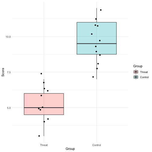
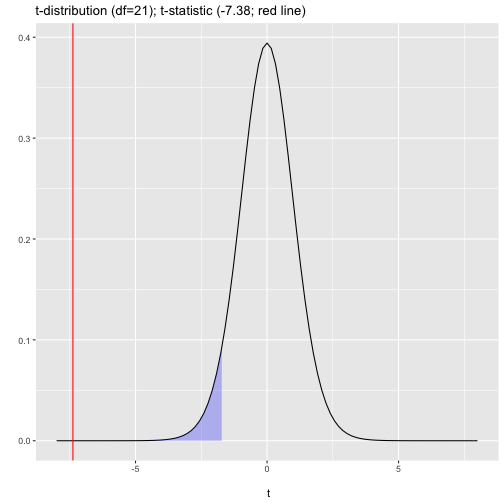
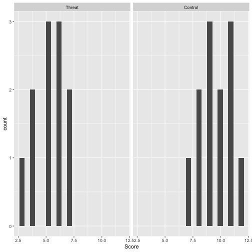
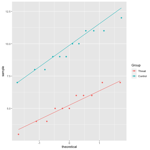
class: center, middle, inverse, title-slide

# Independent t-test
## Data Analysis for Psychology in R 1<br><br>
### dapR1 Team
### Department of Psychology<br>The University of Edinburgh
### AY 2020-2021

---

# Learning Objectives
- Understand when to use an independent sample `$t$`-test

- Understand the null hypothesis for an independent sample `$t$`-test

- Understand how to calculate the test statistic

- Know how to conduct the test in R

- Understand the assumptions for `$t$`-tests

---
# Topics for today

- Recording 1: Conceptual background and introduction to our example

- Recording 2: Calculations and R-functions

- Recording 3: Assumptions and effect size

---
# Purpose & Data
- The independent or Student's `$t$`-test is used when we want to test the difference in mean between two measured groups.

- The groups must be independent:
	- No person can be in both groups.

- Examples:
	- Treatment versus control group in an experimental study.
	- Married versus not married

- Data Requirements
  - A continuously measured variable.
  - A binary variable denoting groups

---
# Hypotheses
- Identical to one-sample, only now we are comparing two measured groups.

- Two-tailed:

$$
`\begin{matrix}
H_0: \bar{x}_1 = \bar{x}_2 \\
H_1: \bar{x}_1 \neq \bar{x}_2
\end{matrix}`
$$

- One-tailed:

$$
`\begin{matrix}
H_0: \bar{x}_1 = \bar{x}_2 \\
H_1: \bar{x}_1 < \bar{x}_2 \\
H_1: \bar{x}_1 > \bar{x}_2
\end{matrix}`
$$

---
# Example
- Example taken from Howell, D.C. (2010). *Statistical Methods for Psychology, 7th Edition*. Belmont, CA: Wadsworth Cengage Learning.

- Data from Aronson, Lustina , Good, Keough , Steele and Brown (1998). Experiment on stereotype threat.
	- Two independent groups college students (n=12 control; n=11 threat condition). 
	- Both samples excel in maths.
	- Threat group told certain students usually do better in the test

---
# Data

```
## # A tibble: 23 x 2
##    Group  Score
##    <fct>  <dbl>
##  1 Threat     7
##  2 Threat     5
##  3 Threat     6
##  4 Threat     5
##  5 Threat     6
##  6 Threat     5
##  7 Threat     4
##  8 Threat     7
##  9 Threat     4
## 10 Threat     3
## # … with 13 more rows
```

---
# Visualizing data 
- We spoke earlier in the course about the importance of visualizing our data.

- Here, we want to show the mean and distribution of scores by group.

- So we want a.....

---
# Visualizing data

.pull-left[

```r
ggplot(data = threat, aes(x = Group, 
                          y = Score, 
                          fill = Group)) +
  geom_boxplot(alpha = 0.3) + 
  geom_jitter(width = 0.1)+
  theme_minimal()  
```
]

.pull-right[
![](dapR1_lec17_independentt_files/figure-html/unnamed-chunk-3-1.png)
]

---
# Hypotheses
- My hypothesis is that the threat group will perform worse than the control group.
  - This is a one-tailed, or directional hypothesis.

- And I will use an `$\alpha= .05$`

---
# t-statistic

$$
t = \frac{\bar{x}_1 - \bar{x}_2}{SE(\bar{x}_1 - \bar{x}_2)}
$$

- Where
  - `$\bar{x}_1$` and `$\bar{x}_2$` are the sample means in each group
  - `$SE(\bar{x}_1 - \bar{x}_2)$` is standard error of the difference

- Sampling distribution is a `$t$`-distribution with `$n-2$` degrees of freedom.

---
# Standard Error Difference
- First calculate the pooled standard deviation.

`$$S_p = \sqrt\frac{(n_1 - 1)s_1^2 + (n_2 - 1)s_2^2}{n_1 + n_2 - 2}$$`

- Then use this to calculate the SE of the difference.

`$$SE(\bar{x}_1 - \bar{x}_2) = S_p \sqrt{\frac{1}{n_1} + \frac{1}{n_2}}$$`

---
class: center, middle
# Time for a break

---
class: center, middle
# Welcome Back!

**OK, we have done all the concepts, now let's do the calculations.**

---
# Calculation
- Steps in my calculations:
  - Calculate the sample mean in both groups.
  - Calculate the pooled SD.
  - Check I know my n.
  - Calculate the standard error.
  - Use all this to calculate `$t$`.

---
# Calculation

```r
calc <- threat %>%
* group_by(Group) %>%
  summarise(
    Mean = round(mean(Score),2),
    SD = round(sd(Score),2),
    N = n()
  ) 
```

```
## # A tibble: 2 x 4
##   Group    Mean    SD     N
## * <fct>   <dbl> <dbl> <int>
## 1 Threat   5.27  1.27    11
## 2 Control  9.58  1.51    12
```

---
# Calculation

```
## # A tibble: 2 x 4
##   Group    Mean    SD     N
## * <fct>   <dbl> <dbl> <int>
## 1 Threat   5.27  1.27    11
## 2 Control  9.58  1.51    12
```

- Calculate pooled standard deviation

`$$S_p = \sqrt\frac{(n_1 - 1)s_1^2 + (n_2 - 1)s_2^2}{n_1 + n_2 - 2} = \sqrt{\frac{10*1.27^2 + 11*1.51^2}{11+12-2}} = \sqrt{\frac{41.21}{21}} = 1.401$$`

---
# Calculation
- Calculate pooled standard deviation

`$$S_p = \sqrt\frac{(n_1 - 1)s_1^2 + (n_2 - 1)s_2^2}{n_1 + n_2 - 2} = \sqrt{\frac{10*1.27^2 + 11*1.51^2}{11+12-2}} = \sqrt{\frac{41.21}{21}} = 1.401$$`

- Calculate the standard error.

`$$SE(\bar{x}_1 - \bar{x}_2) 
= S_p \sqrt{\frac{1}{n_1} + \frac{1}{n_2}} 
= 1.401 \sqrt{\frac{1}{11}+\frac{1}{12}} 
= 1.401 * 0.417 = 0.584$$`

---
# Calculation
- Use all this to calculate `$t$`.

`$$t = \frac{\bar{x}_1 - \bar{x}_2}{SE(\bar{x}_1 - \bar{x}_2)} = \frac{5.27-9.58}{0.584} = -7.38$$`

- Note: When doing hand calculations there might be a small amount of rounding error when we compare to `$t$` calculated in R.
  - In this case, actual value = -7.38

---
# Is my test significant?
- Steps:
  - Calculate my degrees of freedom `$n-2 = 23-2 = 21$`
  - Check my value of `$t$` against the `$t$`-distribution with the appropriate df and make my decision

---
# Is our test significant?

.pull-left[
![](dapR1_lec17_independentt_files/figure-html/unnamed-chunk-7-1.png)

]

.pull-right[

```r
tibble(
  LowerCrit = round(qt(0.05, 21),2),
    Exactp = 1-pt(7.3817, 21)
)
```

```
## # A tibble: 1 x 2
##   LowerCrit      Exactp
##       <dbl>       <dbl>
## 1     -1.72 0.000000146
```

]

---
# Is my test significant?
- So our critical value is -1.72
	- Our t-statistic is larger than this, -7.38.
	- So we reject the null hypothesis.

- `$t$`(21)= -7.38, `$p$` <.05, one-tailed.

---
# In R

```r
res <- t.test(Score ~ Group, 
       var.equal = TRUE,
       alternative = "less",
       data = threat)
```

```
## 
## 	Two Sample t-test
## 
## data:  Score by Group
## t = -7.3817, df = 21, p-value = 1.458e-07
## alternative hypothesis: true difference in means is less than 0
## 95 percent confidence interval:
##       -Inf -3.305768
## sample estimates:
##  mean in group Threat mean in group Control 
##              5.272727              9.583333
```

---
# Write up
An independent sample `$t$`-test was used to assess whether the maths score mean of the control group (12) was higher than that of the stereotype threat group (11). There was a significant difference in test score between the control (Mean=9.58; SD=1.51) and threat (Mean=5.27; SD=1.27) groups ( `$t$`(21)=-7.38, `$p$`< .05, one-tailed). Therefore, we reject the null hypothesis. The direction of effect supports our directional hypothesis and indicates that the threat group performed more poorly than the control group.

---
class: center, middle
# Time for a break

---
class: center, middle
# Welcome Back!

**Next up, checking assumptions and calculating effect size.**

---
# Assumption checks summary

<table class="table table-striped" style="font-size: 18px; width: auto !important; margin-left: auto; margin-right: auto;">
 <thead>
  <tr>
   <th style="text-align:left;">   </th>
   <th style="text-align:left;"> Description </th>
   <th style="text-align:left;"> One-Sample  t-test </th>
   <th style="text-align:left;"> Independent Sample t-test </th>
   <th style="text-align:left;"> Paired Sample t-test </th>
  </tr>
 </thead>
<tbody>
  <tr>
   <td style="text-align:left;"> Normality </td>
   <td style="text-align:left;"> Continuous variable (and difference) is normally distributed. </td>
   <td style="text-align:left;"> Yes (Population) </td>
   <td style="text-align:left;"> Yes (Both groups/ Difference) </td>
   <td style="text-align:left;"> Yes (Both groups/ Difference) </td>
  </tr>
  <tr>
   <td style="text-align:left;"> Tests: </td>
   <td style="text-align:left;"> Descriptive Statistics; Shapiro-Wilks Test; QQ-plot </td>
   <td style="text-align:left;">  </td>
   <td style="text-align:left;">  </td>
   <td style="text-align:left;">  </td>
  </tr>
  <tr>
   <td style="text-align:left;"> Independence </td>
   <td style="text-align:left;"> Observations are sampled independently. </td>
   <td style="text-align:left;"> Yes </td>
   <td style="text-align:left;"> Yes (within and across groups) </td>
   <td style="text-align:left;"> Yes (within groups) </td>
  </tr>
  <tr>
   <td style="text-align:left;"> Tests: </td>
   <td style="text-align:left;"> None. Design issue. </td>
   <td style="text-align:left;">  </td>
   <td style="text-align:left;">  </td>
   <td style="text-align:left;">  </td>
  </tr>
  <tr>
   <td style="text-align:left;"> Homogeneity of variance </td>
   <td style="text-align:left;"> Population level standard deviation is the same in both groups. </td>
   <td style="text-align:left;"> NA </td>
   <td style="text-align:left;"> Yes </td>
   <td style="text-align:left;"> Yes </td>
  </tr>
  <tr>
   <td style="text-align:left;"> Tests: </td>
   <td style="text-align:left;"> F-test </td>
   <td style="text-align:left;">  </td>
   <td style="text-align:left;">  </td>
   <td style="text-align:left;">  </td>
  </tr>
  <tr>
   <td style="text-align:left;"> Matched Pairs in data </td>
   <td style="text-align:left;"> For paired sample, each observation must have matched pair. </td>
   <td style="text-align:left;"> NA </td>
   <td style="text-align:left;"> NA </td>
   <td style="text-align:left;"> Yes </td>
  </tr>
  <tr>
   <td style="text-align:left;"> Tests: </td>
   <td style="text-align:left;"> None. Data structure issue. </td>
   <td style="text-align:left;">  </td>
   <td style="text-align:left;">  </td>
   <td style="text-align:left;">  </td>
  </tr>
</tbody>
</table>

---
# Assumptions
- The independent sample `$t$`-test has the following assumptions:
	- Independence of observations within and across groups.
	- Continuous variable is approximately normally distribution **within both groups**.
	  - Equivalently, that the difference in means is normally distributed.
	- Homogeneity of variance across groups.

---
#  Assumption checks: Normality 
- Descriptive statistics:
	- Skew: No strict cuts for skew.
		- Skew < |1| generally not problematic
		- |1| < skew > |2| slight concern
		- Skew > |2| investigate impact

---
# Histograms

.pull-left[

```r
threat %>%
  ggplot(., aes(x=Score)) +
  geom_histogram(bins = 20) +
  facet_wrap(~ Group)
```

]

.pull-right[
![](dapR1_lec17_independentt_files/figure-html/unnamed-chunk-12-1.png)
]

---
# Skew

```r
library(moments)
threat %>%
  group_by(Group) %>%
  summarise(
    skew = round(skewness(Score),2)
  )
```

```
## # A tibble: 2 x 2
##   Group    skew
## * <fct>   <dbl>
## 1 Threat  -0.23
## 2 Control -0.08
```

---
#  Assumption checks: Normality 
- QQ-plots:
	- Plots the sorted quantiles of one data set (distribution) against sorted quantiles of data set (distribution).
	- Quantile = the percent of points falling below a given value.
	- For a normality check, we can compare our own data to data drawn from a normal distribution

---
# QQ-plots

.pull-left[

```r
threat %>%
  ggplot(., aes(sample = Score, colour = Group)) +
  stat_qq() +
  stat_qq_line()
```

- This looks reasonable in both groups. 
 
]

.pull-right[

![](dapR1_lec17_independentt_files/figure-html/unnamed-chunk-15-1.png)

]

---
#  Assumption checks: Normality 
- Shapiro-Wilks test:
	- Checks properties of the observed data against properties we would expected from normally distributed data.
	- Statistical test of normality.
	- `$H_0$`: data = a normal distribution.
	- `$p$`-value `$< \alpha$` = reject the null, data are not normal.
		- Sensitive to N as all p-values will be.
		- In very large N, normality should also be checked with QQ-plots alongside statistical test.

---
#  Shapiro-Wilks R

```r
con <- threat %>% filter(Group == "Control") %>% select(Score)
shapiro.test(con$Score)
```

```
## 
## 	Shapiro-Wilk normality test
## 
## data:  con$Score
## W = 0.95538, p-value = 0.7164
```

```r
thr <- threat %>% filter(Group == "Threat") %>% select(Score)
shapiro.test(thr$Score)
```

```
## 
## 	Shapiro-Wilk normality test
## 
## data:  thr$Score
## W = 0.93979, p-value = 0.518
```

---
#  Assumption checks: Homogeneity of variance 
- Levene's test:
	- Statistical test for the equality (or homogeneity) of variances across groups (2+).
	- Test statistic is essentially a ratio of variance estimates calculated based on group means versus 
	grand mean.

- The `$F$`-test is a related test that compares the variances of two groups.
  - This test is preferable for `$t$`-test.
	- `$H_0$`: Population variances are equal.
	- `$p$`-value `$< \alpha$` = reject the null, the variances differ across groups.

---
#  F-test R

```r
var.test(threat$Score ~ threat$Group, ratio = 1, conf.level = 0.95)
```

```
## 
## 	F test to compare two variances
## 
## data:  threat$Score by threat$Group
## F = 0.71438, num df = 10, denom df = 11, p-value = 0.6038
## alternative hypothesis: true ratio of variances is not equal to 1
## 95 percent confidence interval:
##  0.2026227 2.6181459
## sample estimates:
## ratio of variances 
##          0.7143813
```

---
#  Violation of homogeneity of variance 
- If the variances differ, we can use a Welch test.

- Conceptually very similar, but we do not use a pooled standard deviation.
	- As such our estimate of the SE of the difference changes
	- As do our degrees of freedom

---
#  Welch test
- If the variances differ, we can use a Welch test.

- Test statistic = same

- SE calculation:

`$$SE(\bar{x}_1 - \bar{x}_2) = \sqrt{\frac{s_1^2}{n_1} + \frac{s_2^2}{n_2}}$$`

- And degrees of freedom (don't worry, not tested)

`$$df = \frac{(\frac{s_1^2}{n_1} + \frac{s_2^2}{n_2})^2}{\frac{(\frac{s_1^2}{n_1})^2}{n_1 -1} + \frac{(\frac{s_2^2}{n_2})^2}{n_2 -1}}$$`

---
# Welch in R

```r
welch <- t.test(Score ~ Group, 
       var.equal = FALSE, #default, only here to highlight difference
       alternative = "less",
       data = threat)
```

---
# Welch in R

```r
welch
```

```
## 
## 	Welch Two Sample t-test
## 
## data:  Score by Group
## t = -7.4379, df = 20.878, p-value = 1.346e-07
## alternative hypothesis: true difference in means is less than 0
## 95 percent confidence interval:
##       -Inf -3.313093
## sample estimates:
##  mean in group Threat mean in group Control 
##              5.272727              9.583333
```

---
#  Cohen's D: Independent t 
- Independent-sample t-test:

$$
D = \frac{\bar{x}_1 - \bar{x}_2}{s_p}
$$

- `$\bar{x}_1$` = mean group 1
-	`$\bar{x}_2$` = mean group 2
-	`$s_p$` = pooled standard deviation

---
# Cohen's D in R

```r
library(effsize)
cohen.d(threat$Score, threat$Group, conf.level = .99)
```

```
## 
## Cohen's d
## 
## d estimate: -3.081308 (large)
## 99 percent confidence interval:
##     lower     upper 
## -4.828153 -1.334463
```

---
# Summary
- Today we have covered:
  - Basic structure of the independent-sample t-test
  - Calculations
  - Interpretation
  - Assumption checks
  - Effect size measures