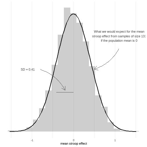
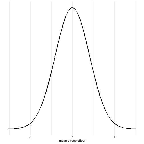
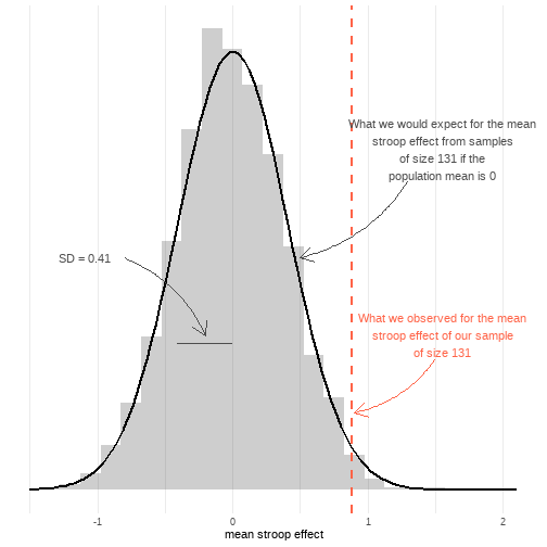
Semester 2, Week 2: Hypothesis Testing & P-values

class: center, middle, inverse, title-slide

# <b>Semester 2, Week 2: Hypothesis Testing & P-values</b>
## Data Analysis for Psychology in R 1
### 
### Department of Psychology<br/>The University of Edinburgh
### AY 2020-2021

---

# Learning objectives

1. Understand null and alternative hypotheses, and how to specify them for a given research question.

2. Understand the concept of a null distribution (via simulation and theoretical).

3. Understand statistical significance and how to calculate p-values from null distributions.  
---
class: inverse, center, middle

# Part 1
## Null and Alternative Hypotheses

---

# Example - Stroop Experiment

Remember this from last semester?

---

# Example - Stroop Experiment

Remember this from last semester?

```r
library(tidyverse)
stroopdata <- read_csv("https://uoepsy.github.io/data/stroopexpt2.csv")
head(stroopdata)
```

```
## # A tibble: 6 x 5
##      id   age matching mismatching stroop_effect
##   <dbl> <dbl>    <dbl>       <dbl>         <dbl>
## 1     1    40    12.6        14             1.39
## 2     2    48    14.8        14.9           0.03
## 3     3    35    15.9        19.6           3.66
## 4     4    47     9.73        4.64         -5.09
## 5     5    27    14.7        14.6          -0.06
## 6     6    55    20.2        17.1          -3.1
```

---

# The ideal

- We have some exact predictions to compare

- Person 1: Mismatching colour words make you 10 seconds slower
    
    - Person 2: Mismatching colour words make you 50 seconds slower
    
{{content}}

- But what happens if it makes you 30 seconds slower?

- Neither is right
    
    - But there is still an effect of the colour mismatch...

---

# The reality

- We have a sample of data

- From which we calculate something (a statistic)

- And we need to use this in some way to make a decision.

- Enter hypothesis testing.

---

# Research Questions vs Hypotheses

.pull-left[

## Research question

- Statement on the expected relations between variables of interest.

- Can be "messy" (not precisely stated)
    
]
.pull-right[
{{content}}
]
    
--

## Statistical hypothesis

- Precise mathematical statement

- **Testable!**

---

# Hypotheses

- The typically applied hypothesis testing framework in psychology has two hypotheses.

- `$H_0$` : the null hypothesis
    
--

- `$H_1$` : the alternative hypothesis
    
---

# Defining `$H_0$`

- The null hypothesis `$H_0$` is the statement that is taken to be true unless there is convincing evidence to the contrary.

--
    
    - `$H_0:$` the status quo
    
--

- In most cases, this is equivalent to assuming there is **"no difference"** or **"no effect"**, or **"What would the result be if only chance were at play?"**

<div style="border-radius: 5px; 
    padding: 20px 20px 10px 20px; 
    margin-top: 20px; 
    margin-bottom: 20px; 
    border-style: solid;">
<center>Example</center>

- If I were trying to guess the playing card you drew from a deck, by chance I would get this right `$\frac{1}{52}$` times.
- My null hypothesis would be that the proportion of guesses which are correct is `$\frac{1}{52} = 0.019$`

---

# Defining `$H_0$`

- Assume that there color-word mismatch has *no influence* on comprehension.
    - And that there was nothing systematic about how participants completed the two conditions (e.g. some did the mismatch condition first, some did the mismatch condition second, and they was randomly allocated)

- What would we expect the mean difference in reaction times between conditions to be? 
    - "for a random participant, if color-word mismatch doesn't affect anything, what's your best guess for the time difference it took them between conditions?"

- Assuming that any differences are just chance, means believing `$\mu_{mismatch-match} = 0$`

<span class="footnote"> `$\mu_{mismatch-match}$` = the population mean difference </span>

---

# Defining `$H_0$`

- `$H_0$` is a very specific hypothesis.

- It states that the population value of a statistic is **equal** to a specific value.

---

# Defining `$H_1$`

- `$H_1$` is the opposing position to `$H_0$`.

- `$H_1$` claims "some other state of the world" is true.

- But is broader with respect to what this might be.

<div style="border-radius: 5px; 
    padding: 20px 20px 10px 20px; 
    margin-top: 20px; 
    margin-bottom: 20px; 
    border-style: solid;">
<center>Example</center>

- We are testing whether I am clairvoyant, and can therefore guess the correct playing card in your hand more often than just by chance. 
- The alternative hypothesis would be that the proportion of guesses which are correct is *greater than* `$\frac{1}{52}$`

---

# Defining `$H_1$`

- `$H_1$` can be **one-sided** or **two-sided**

- Two-sided:
    - `$\mu_{mismatch-match} \neq 0$` 
    
--
 
- One-sided:
    - `$\mu_{mismatch-match} < 0$` 
    - `$\mu_{mismatch-match} > 0$`
    
---

# Defining `$H_1$`

- `$H_1$` can be **one-sided** or **two-sided**

- Two-sided:
    - `$\mu_{mismatch-match} \neq 0$` 
    - "there is *some* difference"
    
--

- One-sided:
    - `$\mu_{mismatch-match} < 0$` 
        - people are quicker for mismatch condition
    - `$\mu_{mismatch-match} > 0$`
        - people are slower for mismatch condition

---

.pull-left[
## Research question

- Statement on the expected relations between variables of interest.

- Can be "messy" (not precisely stated)
    
]
.pull-right[

## Statistical hypothesis

- Precise mathematical statement

- **Testable!**
]

---

.pull-left[
## Research question

- Statement on the expected relations between variables of interest.

- Can be "messy" (not precisely stated)

<div style="border-radius: 5px; 
    padding: 20px 20px 10px 20px; 
    margin-top: 100px; 
    margin-bottom: 20px; 
    border-style: solid;">
Does color-word mismatch interfere with comprehension? 
</div>

]
.pull-right[

## Statistical hypothesis

- Precise mathematical statement

- **Testable!**

<div style="border-radius: 5px; 
    padding: 20px 20px 10px 20px; 
margin-top: 125px; 
    margin-bottom: 20px; 
    border-style: solid;">
    
`$H_0: \mu_{mismatch-match} = 0$`
`$H_1: \mu_{mismatch-match} > 0$`

</div>

]

---
class: inverse, center, middle, animated, rotateInDownLeft

# End of Part 1

---
class: inverse, center, middle

# Part 2
## The Null Distribution

---

# Test Statistic

- A test statistic is the calculation that provides a value in keeping with our research question, in order to test our hypothesis.

- It is calculated on a sample of data.
    
- We have been implicitly talking about such a calculation in our colour-word mismatch example.

- The mean! 
{{content}}
    
<span class="footnote">Aside: Formally the test statistic here is a `$t$`-statistic (we will talk about this in full in a couple of weeks), but we will forego this here to concentrate on the conceptual idea of hypothesis testing</span>

--
    
    - `$\mu_{mismatch-match}$` = The mean in the population
{{content}}
    
--

- `$\bar{x}_{mismatch-match}$` = The mean in our sample

---

# Point estimates

- We have already seen the idea of a point estimate.

- It is simply a value of a statistic calculated in a sample.

```r
stroopdata %>% 
  summarise(
    meanstroop = mean(stroop_effect)
  )
```

```
## # A tibble: 1 x 1
##   meanstroop
##        <dbl>
## 1      0.884
```

- `$\bar{x}_{mismatch-match}$` = 0.88

---

# Null Distribution

<div style="border-radius: 5px; 
    padding: 20px 20px 10px 20px; 
margin-top: 20px; 
    margin-bottom: 20px; 
    background-color:#fcf8e3 !important;">
<center>
<b>Key point</b><br>
A test statistic must have a calculable sampling distribution under the null hypothesis.
</center>
</div>

- ??????
    
--

- Last week (and in the final week of semester 1) we saw how we can construct sampling distributions.

- **IF** the null hypothesis is true, and `$\mu_{mismatch-match} = 0$`, what would the variation around `$\bar{x}_{mismatch-match}$`.
 
---
 
# Null Distribution

.pull-left[
![](dapR1_lec12_nhstpval_files/figure-html/unnamed-chunk-4-1.png)
]
.pull-right[
{{content}}
]

How did we get here??
{{content}}

1. Simulation! 
{{content}}

2. Theory!
{{content}}

---

# Simulating the Null Distribution

.pull-left[
generate (e.g. bootstrap) many samples of 131 with mean 0, and look at all their means... 
{{content}}
]
--

```r
source("https://uoepsy.github.io/files/rep_sample_n.R")
stroopdata <- 
  stroopdata %>% 
  mutate(
    shifted = stroop_effect - mean(stroop_effect)
  )

bootstrap_dist <- 
  rep_sample_n(stroopdata, n = 131, samples = 2000, replace = TRUE) %>%
  group_by(sample) %>%
  summarise(
    resamplemean = mean(shifted)
  ) -> bootstrap_dist

sd(bootstrap_dist$resamplemean)
```

```
## [1] 0.4101
```

.pull-right[

```r
ggplot(bootstrap_dist, 
       aes(x = resamplemean))+
  geom_histogram()
```

<img src="dapR1_lec12_nhstpval_files/figure-html/unnamed-chunk-6-1.png" width="504" height="350px" />
]

---

# Theorising about the Null Distribution

.pull-left[

- `$SE = \frac{\sigma}{\sqrt{n}}$`

```r
sd(stroopdata$stroop_effect)
```

```
## [1] 4.737
```

```r
nrow(stroopdata)
```

```
## [1] 131
```

```r
sd(stroopdata$stroop_effect) / sqrt(131)
```

```
## [1] 0.4139
```
]

.pull-right[
![](dapR1_lec12_nhstpval_files/figure-html/unnamed-chunk-8-1.png)
]

---

# Null Distribution

---
class: inverse, center, middle, animated, rotateInDownLeft

# End of Part 2

---
class: inverse, center, middle

# Part 3
## Probability and the Null

---

## Probability and the Null

.pull-left[
![](dapR1_lec12_nhstpval_files/figure-html/unnamed-chunk-10-1.png)
]
.pull-right[
{{content}}
]

- To recap the last 5 weeks of semester 1, the area under the curve provides us with probability. 
{{content}}

- We can calculate the probability of values more extreme than where the red line (our sample estimate), is on our x-axis.  
{{content}}

- This probability is what is referred to as the `$p$`-value.

---

# p-value

- The `$p$`-value represents the chance of obtaining a statistic as extreme or more extreme than the observed statistic, **if the null hypothesis were true**.

- Think of it as `$P(Data | Hypothesis)$`  
    ("the probability of our data *given* the null hypothesis").

---

# Calculating the p-value

.pull-left[
**Simulation**  
`$SE_{bootstrap} =$` 0.41

```r
bootstrap_se = sd(bootstrap_dist$resamplemean)
bootstrap_se
```

```
## [1] 0.4101
```
What proportion of resample means are > our observed mean 0.88?

```r
sum(bootstrap_dist$resamplemean >= mean(stroopdata$stroop_effect)) / 2000
```

```
## [1] 0.0155
```

]
.pull-right[
**Theory**  
`$SE = \frac{\sigma}{\sqrt{n}} =$` 0.41

```r
formula_se = sd(stroopdata$stroop_effect) / sqrt(131)
formula_se
```

```
## [1] 0.4139
```
For a normal distribution with mean 0 and sd 0.41, what is the probability of observing a value greater than our observed mean 0.88?

```r
1-pnorm(mean(stroopdata$stroop_effect), mean = 0, sd = formula_se)
```

```
## [1] 0.01632
```

]

---

# What about the other extreme?

- Depends on our hypothesis.  
{{content}}

.footnote[See <a href="https://uoepsy.github.io/dapr1/lectures/recap_pvalues.pdf" target="_blank">here</a> for a useful reminder.]

- If our hypothesis is **one-tailed** (e.g., `$\mu < 0$` or `$\mu > 0$`), then we're only interested in one tail. 
- If our hypothesis is **two-tailed** (e.g., `$\mu \neq 0$`), then we're interested in both tails.  
{{content}}

- But sampling distrubutions are normal (and so symmetric), meaning that 2 `$\times$` one tail will give us the probability of observing a statistic at least extreme *in either direction*.

---

# Making a decision

- So we know the probability of getting a value at least as extreme as our point estimate, given the sampling distribution for the null.

- How can we evaluate it to inform our beliefs?

- We do this by assigning a significance level, or `$\alpha$` level.

- `$\alpha$` is the cut-off point.  
    - If our `$p$`-value is `$< \alpha$` we make one decision. 
    - If our `$p$`-value is `$\geq \alpha$` we make another decision
    
--

- We typically use `$\alpha$` = 0.05

---

# Interpreting our result

- `$p$`-value is `$< \alpha$`: We reject the null hypothesis

- `$p$`-value is `$\geq \alpha$`: We fail to reject the null hypothesis

- Odd language:  
    - We don't "accept" the null? We just have no reason not to believe it.
    - We don't "accept" the alternative? We never really tested the alternative (our sampling distribution was based around the null)

---

# Interpreting our result

### Alternative

- `$p$`-value is `$< \alpha$` / `$\geq \alpha$` : We **reject**/**maintain** the null hypothesis.

- "maintaining" and "rejecting" is not about whether an hypothesis is *objectively true*, it is about our belief in it. 
    - I can "maintain" that the earth is flat

---

## Summary

- Structure of a Hypothesis Test

1. A hypothesis
    2. A hypothesis test
    3. Test statistic
    4. Observed test statistic (point estimate from sample)
    5. Null distribution
    6. `$p$`-value
    7. `$p$`-value `$< \alpha$` / `$\geq$` Significance level ($\alpha$)

---

class: inverse, center, middle, animated, rotateInDownLeft

# End