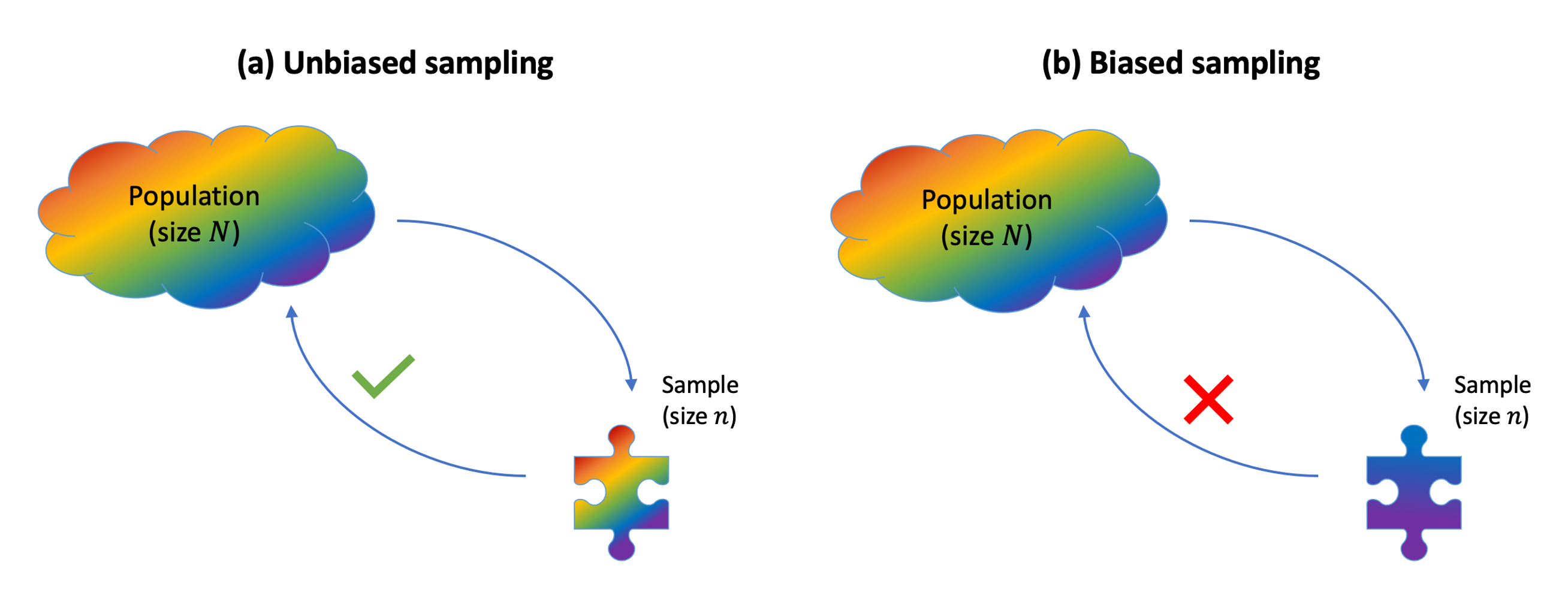
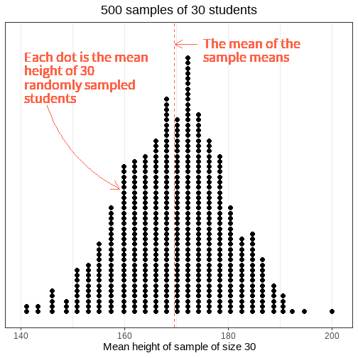
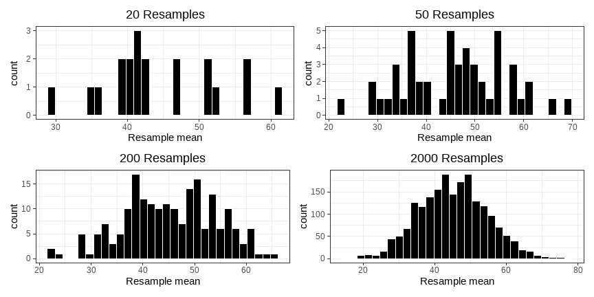
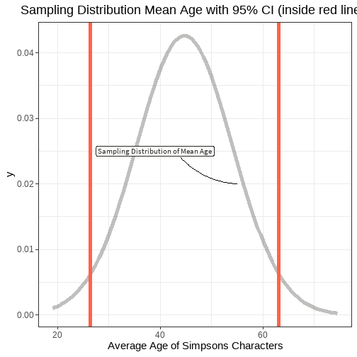
class: center, middle, inverse, title-slide # <b>Semester 2, Week 1: Bootstrapping and Confidence Intervals</b> ## Data Analysis for Psychology in R 1 ### ### Department of Psychology<br/>The University of Edinburgh ### AY 2020-2021 --- # This Week's Learning Objectives 1. Understand how bootstrap resampling with replacement can be used to approximate a sampling distribution. 2. Understand how the bootstrap distribution can be used to construct a range of highly plausible values (a confidence interval). 3. Understand the link between simulation-based standard errors and theory-based standard errors. --- class: inverse, center, middle # Part 1 ## Bootstrapping --- # Samples <center> <img src="jk_img_sandbox/statistical_inference.png" width="600" height="500" /> </center> --- # Good Samples - If a sample of `\(n\)` is drawn at **random**, it will be unbiased and representative of `\(N\)` - Point estimates from such samples will be good estimates of the population parameter. - Without the need for census.  --- # Recap on sampling distributions .pull-left[ - We have a population. - We take a sample of size `\(n\)` from it, and calculate our statistic - The statistic is our estimate of the population parameter. - We do this repeatedly, and we can construct a sampling distribution. - The mean of the sampling distribution will be a good approximation to the population parameter. - To quantify sampling variation we can refer to the standard deviation of the sampling distribution (the **standard error**) ] .pull-right[ {{content}} ] -- + University students {{content}} -- + We take a sample of 30 students, calculate the mean height. {{content}} -- + This is our estimate of the mean height of all university students. {{content}} -- + Do this repeatedly (take another sample of 30, calculate mean height). {{content}} -- + The mean of these sample means will be a good approximation of the population mean. {{content}} -- + To quantify sampling variation in mean heights of 30 students, we can refer to the standard deviation of these sample means. {{content}} --- # Practical problem: .pull-left[ <!-- --> ] .pull-right[ - This process allows us to get an estimate of the sampling variability, **but is this realistic?** - Can I really go out and collect 500 samples of 30 students from the population? - Probably not... {{content}} ] -- - So how else can I get a sense of the variability in my sample estimates? --- .pull-left[ ## Solution 1 ### Theoretical - Collect one sample. - Estimate the Standard Error using the formula: <br> `\(\text{SE} = \frac{\sigma}{\sqrt{n}}\)` ] .pull-right[ ## Solution 2 ### Bootstrap - Collect one sample. - Mimick the act of repeated sampling from the population by repeated **resampling with replacement** from the original sample. - Estimate the standard error using the standard deviation of the distribution of **resample** statistics. ] --- # Resampling 1: The sample .pull-left[ <img src="jk_img_sandbox/sample.png" width="350" /> Suppose I am interested in the mean age of all characters in The Simpsons, and I have collected a sample of `\(n=10\)`. {{content}} ] -- + The mean age of my sample is 44.9. -- .pull-right[ ``` ## # A tibble: 10 x 2 ## name age ## <chr> <dbl> ## 1 Homer Simpson 39 ## 2 Ned Flanders 60 ## 3 Chief Wiggum 43 ## 4 Milhouse 10 ## 5 Patty Bouvier 43 ## 6 Janey Powell 8 ## 7 Montgomery Burns 104 ## 8 Sherri Mackleberry 10 ## 9 Krusty the Clown 52 ## 10 Jacqueline Bouvier 80 ``` ```r simpsons_sample %>% summarise(mean_age = mean(age)) ``` ``` ## # A tibble: 1 x 1 ## mean_age ## <dbl> ## 1 44.9 ``` ] --- # Resampling 2: The **re**sample .pull-left[ I randomly draw out one person from my original sample, I note the value of interest, and then I put that person "back in the pool" (i.e. I sample with replacement). <br> <br> <img src="jk_img_sandbox/resample1.png" width="350" /> ] .pull-right[ ``` ## # A tibble: 1 x 2 ## name age ## <chr> <dbl> ## 1 Chief Wiggum 43 ``` ] --- # Resampling 2: The **re**sample .pull-left[ Again, I draw one person at random again, note the value of interest, and replace them. <br> <br> <img src="jk_img_sandbox/resample2.png" width="350" /> ] .pull-right[ ``` ## # A tibble: 2 x 2 ## name age ## <chr> <dbl> ## 1 Chief Wiggum 43 ## 2 Ned Flanders 60 ``` ] --- # Resampling 2: The **re**sample .pull-left[ And again... <br> <br> <br> <img src="jk_img_sandbox/resample3.png" width="350" /> ] .pull-right[ ``` ## # A tibble: 3 x 2 ## name age ## <chr> <dbl> ## 1 Chief Wiggum 43 ## 2 Ned Flanders 60 ## 3 Janey Powell 8 ``` ] --- # Resampling 2: The **re**sample .pull-left[ And again... <br> <br> <br> <img src="jk_img_sandbox/resample4.png" width="350" /> ] .pull-right[ ``` ## # A tibble: 4 x 2 ## name age ## <chr> <dbl> ## 1 Chief Wiggum 43 ## 2 Ned Flanders 60 ## 3 Janey Powell 8 ## 4 Ned Flanders 60 ``` ] --- # Resampling 2: The **re**sample .pull-left[ Repeat until I have a the same number as my original sample ( `\(n = 10\)` ). <br> <br> <img src="jk_img_sandbox/resample.png" width="350" /> {{content}} ] .pull-right[ ``` ## # A tibble: 10 x 2 ## name age ## <chr> <dbl> ## 1 Chief Wiggum 43 ## 2 Ned Flanders 60 ## 3 Janey Powell 8 ## 4 Ned Flanders 60 ## 5 Patty Bouvier 43 ## 6 Chief Wiggum 43 ## 7 Jacqueline Bouvier 80 ## 8 Montgomery Burns 104 ## 9 Sherri Mackleberry 10 ## 10 Patty Bouvier 43 ``` ] -- - This is known as a **resample** {{content}} -- - The mean age of the resample is 49.4 --- # Bootstrapping: Resample₁, ..., Resample_k - If I repeat this whole process many times, say k=1000, I will have 1000 means from 1000 resamples. - Note these are entirely derived from the original sample. - This is known as called **bootstrapping**, and the resultant distribution of statistics (in our example, the distribution of 1000 resample means) is known as a **bootstrap distribution.** <div style="border-radius: 5px; padding: 20px 20px 10px 20px; margin-top: 20px; margin-bottom: 20px; background-color:#fcf8e3 !important;"> **Bootstrapping** The process of resampling *with replacement* from the original data to generate a multiple resamples of the same `\(n\)` as the original data. --- # Bootstrap distribution - Start with an initial sample of size `\(n\)`. - Take `\(k\)` resamples (sampling with replacement) of size `\(n\)`, and calculate your statistic on each one. - As `\(k\to\infty\)`, the distribution of the `\(k\)` resample statistics begins to approximate the sampling distribution. - Note, this is just the same exercise as we did with samples from the population in previous weeks. --- # k = 20, 50, 200, 2000, ... <!-- --> --- # Bootstrap Standard Error - Previously we spoke about the standard error as the measure of sampling variability. -- - We stated that this was just the SD of the sampling distribution. -- - In the same vein, we can calculate a bootstrap standard error - the SD of the bootstrap distribution. <!-- --> --- class: inverse, center, middle, animated, rotateInDownLeft # End of Part 1 --- class: inverse, center, middle # Part 2 ## Confidence Intervals --- # Confidence interval - Remember, usually we do not know the value of a population parameter. - We are trying to estimate this from our data. -- - A confidence interval defines a plausible range of values for our population parameter. - To estimate we need: - A **confidence level** - A measure of sampling variability (e.g. SE/bootstrap SE). --- # Confidence interval & level <div style="border-radius: 5px; padding: 20px 20px 10px 20px; margin-top: 20px; margin-bottom: 20px; background-color:#fcf8e3 !important;"> **x% Confidence interval** across repeated samples, [x]% confidence intervals would be expected to contain the true population parameter value.</div> x% is the *confidence level*. Commonly, you will use and read about **95%** confidence intervals. If we were to take 100 samples, and calculate a 95% CI on each of them, approx 95 of them would contain the true population mean. -- - What are we 95% confident *in?* - We are 95% confident that our interval [lower, upper] contains the true population mean. - This is subtly different from saying that we are 95% confident that the true mean is inside our interval. The 95% probability is related to the long-run frequencies of our intervals. --- # Simple Visualization .pull-left[ <!-- --> ] .pull-right[ - The confidence interval works outwards from the centre - As such, it "cuts-off" the tails. - E.g. the most extreme estimates will not fall within the interval ] --- # Calculating CI - We want to identify the upper and lower bounds of the interval (i.e. the red lines from previous slide) - These need to be positioned so that 95% of all possible sample mean estimates fall within the bounds. --- # Calculating CI: 68/95/99 Rule - Remember that sampling distributions become normal... - There are fixed properties of normal distributions. -- - Specifically: - 68% of density falls within 1 SD of the mean - 95% of density falls with 1.96 SD of the mean - 99.7% of density falls within 3 SD of the mean - Remember the standard error = SD of the bootstrap (or sampling distribution)... --- # Calculating CI - ... the bounds of the 95% CI for a mean are: $$ \text{Lower Bound} = mean - 1.96 \cdot SE $$ $$ \text{Upper Bound} = mean + 1.96 \cdot SE $$ --- # Calculating CI - Example ```r simpsons_sample <- read_csv("https://uoepsy.github.io/data/simpsons_sample.csv") mean(simpsons_sample$age) ``` ``` ## [1] 44.9 ``` --- # Calculating CI - Example ```r # Theoretical approach mean(simpsons_sample$age) - 1.96*(sd(simpsons_sample$age)/sqrt(10)) ``` ``` ## [1] 25.47 ``` ```r mean(simpsons_sample$age) + 1.96*(sd(simpsons_sample$age)/sqrt(10)) ``` ``` ## [1] 64.33 ``` --- # Calculating CI - Example ```r # Bootstrap Approach source('https://uoepsy.github.io/files/rep_sample_n.R') resamples2000 <- rep_sample_n(simpsons_sample, n = 10, samples = 2000, replace = TRUE) bootstrap_dist <- resamples2000 %>% group_by(sample) %>% summarise(resamplemean = mean(age)) sd(bootstrap_dist$resamplemean) ``` ``` ## [1] 9.334 ``` ```r mean(simpsons_sample$age) - 1.96*sd(bootstrap_dist$resamplemean) ``` ``` ## [1] 26.6 ``` ```r mean(simpsons_sample$age) + 1.96*sd(bootstrap_dist$resamplemean) ``` ``` ## [1] 63.2 ``` --- # Sampling Distributions and CIs are not just for means. For a 95% Confidence Interval around a statistic: $$ \text{Lower Bound} = statistic - 1.96 \cdot SE $$ $$ \text{Upper Bound} = statistic + 1.96 \cdot SE $$ --- # Summary - Good samples are representative, random and unbiased. - Bootstrap resampling is a tool to construct a *bootstrap distribution* of any statistic which, with sufficient resamples, will approximate the *sampling distribution* of the statistic. - Confidence Intervals are a tool for considering the plausible value for an unknown population parameter. - We can use bootstrap SE to calculate CI. --- class: inverse, center, middle, animated, rotateInDownLeft # End